-
Paper Information
- Next Paper
- Previous Paper
- Paper Submission
-
Journal Information
- About This Journal
- Editorial Board
- Current Issue
- Archive
- Author Guidelines
- Contact Us
International Journal of Statistics and Applications
p-ISSN: 2168-5193 e-ISSN: 2168-5215
2017; 7(2): 73-92
doi:10.5923/j.statistics.20170702.03

Competitive Assessment of Two Variance Weighted Gradient (VWG) Methods with Some Standard Gradient and Non-Gradient Optimization Methods
 Abstract
 Reference
 Full-Text PDF
 Full-text HTML
Otaru O. A. P., Iwundu M. P.
Department of Mathematics and Statistics, University of Port Harcourt, Port Harcourt, Nigeria
Correspondence to: Iwundu M. P., Department of Mathematics and Statistics, University of Port Harcourt, Port Harcourt, Nigeria.
| Email: |  |
Copyright © 2017 Scientific & Academic Publishing. All Rights Reserved.
This work is licensed under the Creative Commons Attribution International License (CC BY).
http://creativecommons.org/licenses/by/4.0/

A competitive assessment of the performance of two Variance Weighted Gradient (VWG) methods with some gradient and non-gradient optimization methods is considered for optimizing polynomial response surfaces. The variance weighted gradient methods could involve several response surfaces defined on joint feasible regions having same constraints or several response surfaces defined on disjoint feasible regions having different constraints. The gradient and non-gradient optimization methods include Quasi-Newton (GN), Genetic Algorithm (GA), Mesh Adaptive Search (MADS) and Generalized Pattern Search (GPS) methods. The variance weighted gradient methods perform considerably and comparatively well and require few iterative steps to convergence.
Keywords: Response Surfaces, Optimization, Gradient Method, Non-Gradient Method, Weighted Gradients methods
Cite this paper: Otaru O. A. P., Iwundu M. P., Competitive Assessment of Two Variance Weighted Gradient (VWG) Methods with Some Standard Gradient and Non-Gradient Optimization Methods, International Journal of Statistics and Applications, Vol. 7 No. 2, 2017, pp. 73-92. doi: 10.5923/j.statistics.20170702.03.
Article Outline
1. Introduction
- Gradient and non-gradient methods are popular techniques used in optimizing response functions. They have been very helpful in handling optimization of single objective functions. In the presence of multi-objective functions, the popularly used one-at-a-time optimization techniques become time consuming. In fact, the challenge in getting a good guess of starting point introduces cycling and sometime lack of convergence. The Gradient and non-gradient methods include Newton Method (NM), Guasi-Newton Method (GNM), Genetic Algorithm (GA), Mesh Adaptive Search (MADS) and Generalized Pattern Search (GPS) methods, etc. These methods could readily be seen in statistical software and thus, easy to use in handling optimization problems. As documented in Patil and Verma (2009), the Newton method was developed by Newton in 1669 and was later improved by Raphson in 1690 and hence popularly referred to as Newton-Raphson’s iterative algorithm. NM is the commonly applied gradient-based method for optimizing polynomial function when the first and second derivative of the function is explicitly available. It assumes that the function can be locally approximated as a quadratic in the region around the optimum. Newton method requires computation of Hessian matrix and the convergence of the method is slow. Davidon (1959) developed the Quasi Newton Method (QNM) which was later popularized by Fletcher and Powell (1963). The Quasi Newton Method can be used if the Hessian matrix is unavailable or too expensive to compute at all iterations. Thus the Quasi Newton Method helps to reduce computational rigor involved in the Newton method. Commonly used Quasi Newton algorithms are the SR1 formular, the BHHH method, the BFGS method and the L-BFGS method. Holland (1975) developed Genetic Algorithms (GAs) for linear and non-linear functions optimization. The algorithm solves both constrained and unconstrained optimization problems using natural procedure that imitates biological evolution. Genetic Algorithms can be used to solve problems where standard optimization techniques do not apply as well as problems in which the objective function is discontinuous or non-linear. Pattern search algorithms can also be employed in getting optimal solutions. The generalized pattern search (GPS) for unconstrained optimization problems is due to Torczon (1997) and does not require information about the gradient or higher derivative to arrive at the optimal point. Audet and Dennis Jr (2006) developed the Mesh Adaptive Direct Search (MADS) as a class of algorithm that extends the generalized pattern search. Both algorithms compute a sequence of points that approach the optimal solutions. Abramson et.al (2009) applied the Mesh adaptive direct search in solving constrained mixed variable optimization problems in which variables may be continuous or categorical. The gradient-free class of Mesh adaptive direct search algorithm is called Mixed Variable MADS abbreviated MV-MADS. Audit et.al (2010) introduced MULTIMAD, a multi-objective Mesh adaptive direct search optimization algorithm. For more on the Gradient and non-gradient methods, see Audet and Dennis Jr (2009), Audet et.al (2014), Dolan et.al (2003), Goldberg (1989), Kolda et.al (2003), Lewin (1994a), Lewin (1994b), Lewis and Torczon (2000).Iwundu et.al (2014) developed an iterative variance weighted gradient procedure that can simultaneously optimize multi-objective functions defined on the same region or having the same constraints. When the constraints are different and the regions are disjoint, a projection scheme that allows the projection of design points from one region to another is used. The performance of the variance weighted gradient method due to Iwundu et al. (2014) and its modified projection scheme technique shall be compared with the gradient-based QNM and non-gradient optimization methods, namely, GA, MADS and GPS. The basic algorithmic steps of the variance weighted gradient methods are presented in section 2.
2. Methodology
- We present the algorithmic steps of the variance weighted gradient method for joint feasible region as well as for disjoint feasible region.
2.1. Variance Weighted Gradient (VWG) Method for Joint Feasible Regions with Same Constraints
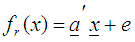
- Let
 be an n-variate, p-parameter polynomial functions of degree m defined by constraints on the same feasible region, given by
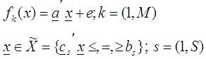 | (1) |
 is a p-component vector of known coefficient,
  is the random error component assumed normally and independently distributed with zero mean and constant variance,
  is a component vector of known coefficients and
  is a scalar for s number of constraints. The Variance Weighted Gradient (VWG) method for joint feasible regions with same constraints is defined by the following iterative steps:i) Obtain N support points
 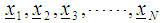 from
from  ii) Define the design measures
  which is made up of N support points such that
 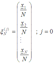 where
where  support points are spread evenly in
  iii) From the support point l (1, N) that makes up the design measure, compute the starting points as.
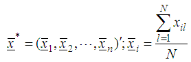 iv) Obtain the n-component gradient vector for the kth function.
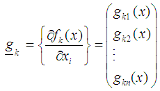 where
where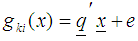 is an
is an  degree polynomial;
 is a t-component vector of known coefficients v) Compute the corresponding kth gradient vector, by substituting each l design point to the gradient function
  as
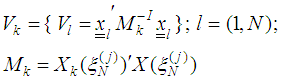
as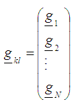 vi) Using the gradient function and design measures obtain the corresponding design matrices
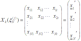 In order to form the design matrix
  a single polynomial that combines the respective gradient function
  associated with each response function
  is
is  vii) Compute the variances of each l design point
  for the kth function as
 viii) Obtain the direction vector for the kth function as
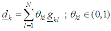 and the normalize direction vector
 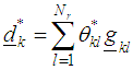 such that
  ix) Compute the step-length
  as
as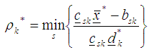 x) With
  and
and  make a move to
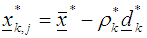 xi) To make a next move set
  and define the design measure as
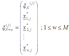 and repeat the process from step (iii) then obtain
 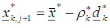 xii) If
 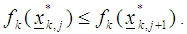 where
where  is the kth function at the jth step and
  is the kth function at the next (j+1)th step.then set the optimizers as
  and STOP. Else, set
  and repeat the process from (iii).
2.2. Variance Weighted Gradient (VWG) Method for Disjoint Feasible Regions with Different Constraints
- Let
 | (2) |
 supported by s constraints. Such that
 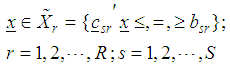 where
where  is a p-component vector of known coefficients, independent random variable
  and
and  is the random error component assumed normally and independently distributed with zero mean and constant variance. While
  is a component vector of know coefficients and
  is a scalar for s number of constraints in the rth region.The Variance Weighted Gradient (VWG) method for disjoint feasible regions, with different Constraints, is given by the following sequential steps:i) From
  obtain the design measures
  which are made up of support points from respective regions such that
 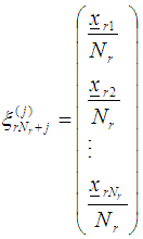 where
where  support points are spread evenly in
  ii) From the support points that make up the design measure compute R starting points as, the arithmetic mean vectors.
 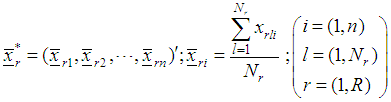 iii) Obtain the n-component gradient function for the rth region.
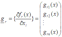 where
where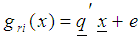 is an
is an  degree polynomial ;
 is a t-component vector of known coefficients iv) Compute the corresponding r gradient vectors, by substituting each design point defined on the rth region to the gradient function
  as
as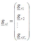 v) Using the gradient function and design measures obtain the corresponding design matrices
 In order to form the design matrix
  a single polynomial that combines the respective gradient function
  associated with each response function
  is
is  vi) Compute the variances of each l design point
  defined on the rth region as
 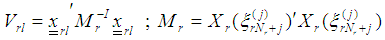 vii) Obtain the direction vector in the rth region as
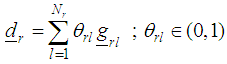 and the normalize direction vector
 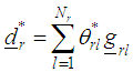 such that
  viii) Compute the step-length
  as
as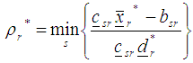 with
with  and
and  make a move to
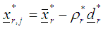 using
using  evaluate the projection operator
  as
as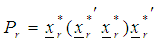 and obtain the projector optimizers for each region
  as
as 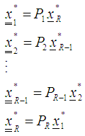 ix) To make a next move set
  and define the design measure as
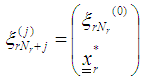 and repeat the process from step (ii) then obtain
 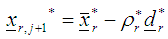 x) If
x) If 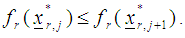 where
where  is the rth feasible region at the jth step and
  is the rth feasible region at the next j+1th step.then set the optimizers as
  and STOP. Else, set
  and repeat the process from (ii).
3. Results
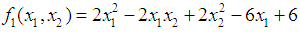
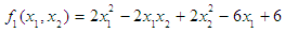
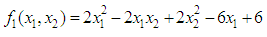
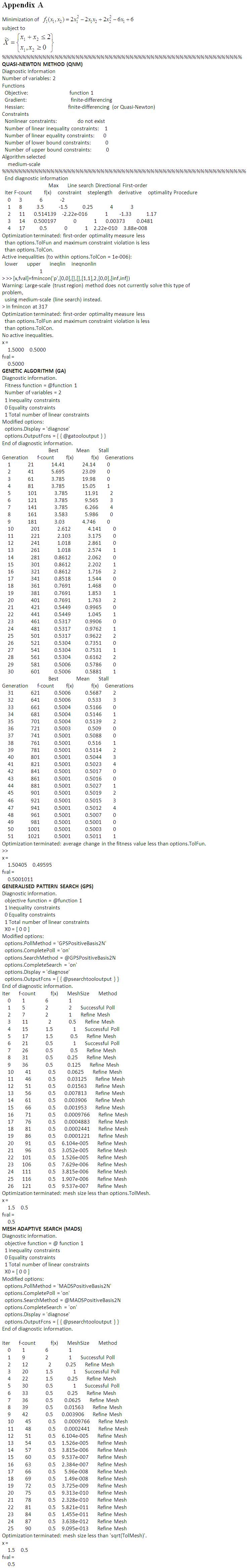
- In comparing the Variance Weighted Gradient (VWG) algorithms with standard gradient and non-gradient methods, we consider the optimization problems;Problem 1Minimize
 subject to
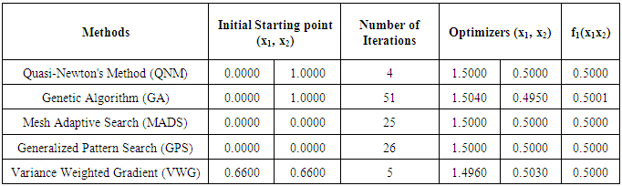
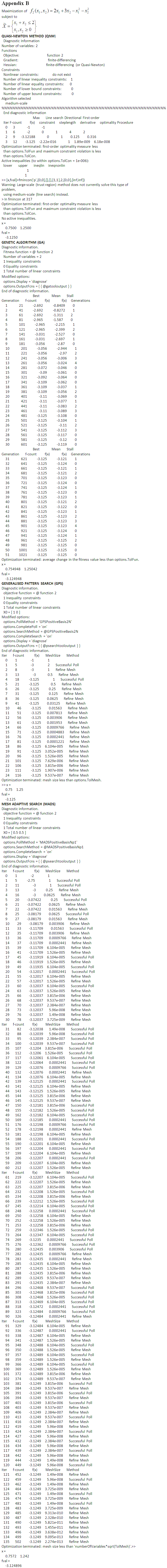
 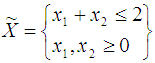 (Ghadle and Pawar, 2015)and Maximize
 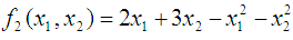 subject to
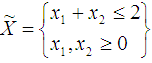 (Hillier and Lieberman, 2001).The solution to the minimization problem
 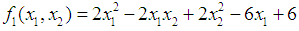 using the Variance Weighted Gradient (VWG) method is
 and
and  from an initial starting point,
  Similarly, the solution to the maximization problem
  using the Variance Weighted Gradient (VWG) method is

 and
and  from an initial starting point,
  QN, GA, MADS and GPS methods obtained the respective solutions


 to the minimization problem
  from respective initial guess value,


 Similarly, QN, GA, MADS and GPS methods obtained the respective solutions
 to the maximization problem
  from respective initial guess value,


 The summary results are as tabulated in Tables 1 and 2.
|
 Subject to
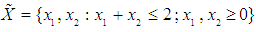
|
 Subject to
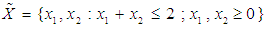
 subject to
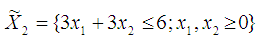 (Hillier and Lieberman, 2001)andMaximize
 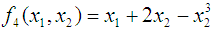 subject to
 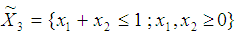 (Hillier and Lieberman, 2001)The solution to the maximization problem
 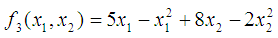 using the Variance Weighted Gradient (VWG) method is

 and
and  from an initial starting point,
  Similarly, the solution to the maximization problem
  using the Variance Weighted Gradient (VWG) method is

 and
and  from an initial starting point,
  QN, GA, MADS and GPS methods obtained the respective solutions


 from respective initial guess value,


 to the maximization problem
 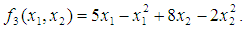 In like manner, QN, GA, MADS and GPS methods obtained the respective solutions for


 from respective initial guess value,

 to the maximization problem
  The summary results are as tabulated in Tables 3 and 4.
|
 Subject to
|
 Subject to
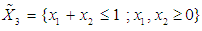
4. Discussion of Results
- In minimizing
 subject to
  and
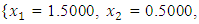
and  the Quasi-Newton Method (QNM) with the initial guess starting point (0.0000, 1.0000) locates the optimizer (1.5000, 0.5000) in 4 iterations with a response function value of 0.5000. Genetic Algorithm (GA) with initial guess starting points (0.0000, 1.0000) locates the optimizer (1.5040, 0.4950) in 51 iterations with a response function value of 0.5001. The Mesh Adaptive Search (MADS) and Generalized Pattern Search (GPS) methods, with initial guess starting point (0.0000, 0.0000), locate the same optimizer (1.5000, 0.5000) with a response function value of 0.5000 in 25 and 26 iterations, respectively. The Variance Weighted Gradient Method (VWG) obtained optimizers (1.4960, 0.5030) in 5 iterations, with a response function value of 0.5000 from an initial optimum starting point (0.66, 0.66).In maximizing
 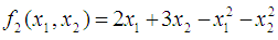 subject to
  and
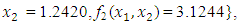
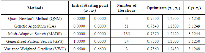
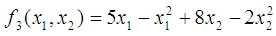
and  the Quasi-Newton Method (QNM) method, with the initial guess starting point (0.0000, 0.0000) locates the optimizer (0.7500, 1.2500) in 3 iterations with a response function value of 3.1250. The Genetic Algorithm (GA), with the initial guess starting point (0.0000, 0.0000) locates the optimizer (0.7540, 1.2500) in 51 iterations with a response function value of 3.1249. The Mesh Adaptive Search (MADS) method, with the initial guess starting point (0.0000, 0.0000) locates the optimizer (0.7570, 1.2420) in 135 iterations with a response function value of 3.1244. The Generalized Pattern Search (GPS) method, with the initial guess starting point (1.0000, 0.0000) locates the optimizer (0.7500, 1.2500) in 24 iterations with a response function value of 3.1250. The Variance Weighted Gradient Method (VWG) obtained optimizers (0.7560, 1.2430) in 3 iterations, with a response function value of 3.1249 from an initial optimum starting point (0.66, 0.66). In maximizing
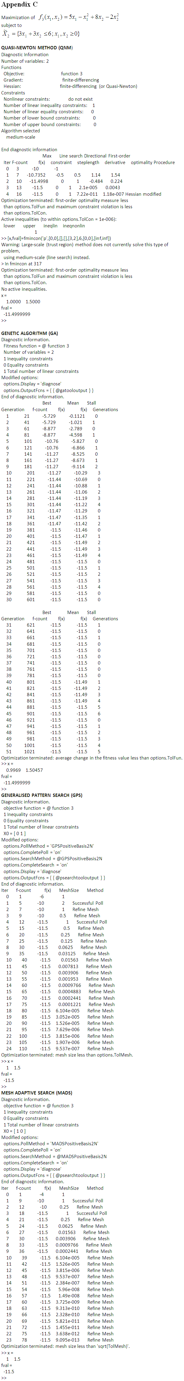
  subject to
  and
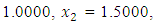
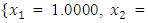
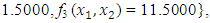
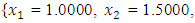
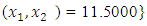
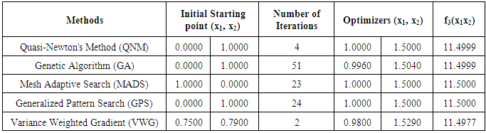
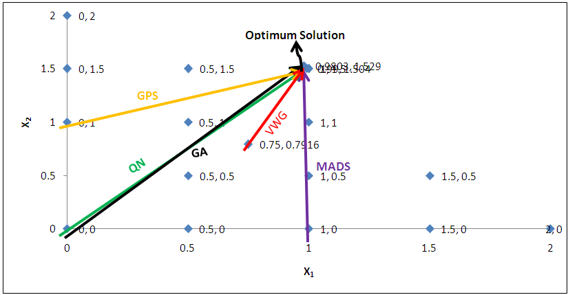
and  , the Quasi-Newton Method (QNM) with the initial guess starting point (0.0000, 1.0000) locates the optimizer (1.0000, 1.5000) in 4 iterations with a response function value of 11.4999. Genetic Algorithm (GA) with initial guess starting point (0.0000, 1.0000) locates the optimizer (0.9960, 1.5040) in 51 iterations, with response function value 11.4999. The Mesh Adaptive Search (MADS) method with initial guess starting point (1.0000, 0.0000) locates the optimizer (1.0000, 1.5000) in 23 iterations, with response function value 11.5000. The Generalized Pattern Search (GPS) method with initial guess starting point (0.0000, 1.0000) locates the optimizer (1.0000, 1.5000) in 24 iterations, with response function value of 11.5000. The Variance Weighted Gradient Method (VWG) obtained optimizers (0.9800, 1.5290) from an initial optimum starting point (0.7500, 0.7900) in 2 iterations, with response function value of 11.4977.
 | Figure 1. Optimum Point of 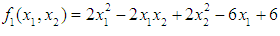 Subject to Subject to  |
 | Figure 2. Optimum Point of  Subject to Subject to  |
 | Figure 3. Optimum Point of  Subject to Subject to  |
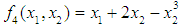
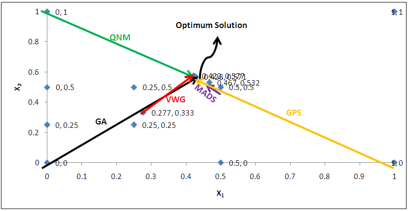 | Figure 4. Optimum Point of  subject to subject to  |
 subject to
  and
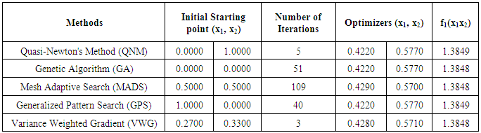
and  , the Quasi-Newton Method (QNM) with the initial guess starting point (0.0000, 1.0000) locates the optimizer (0.4220, 0.5770) in 5 iterations with a response function value of 1.3849. Genetic Algorithm (GA) with the initial guess starting point (0.0000, 0.0000) locates the optimizer (0.4220, 0.5770) in 51 iterations with a response function value of 1.3849. The Mesh Adaptive Search (MADS) method with the initial guess starting point (0.5000, 0.5000) locates the optimizer (0.4290, 0.5770) in 109 iterations with a response function value of 1.3848. The Generalized Pattern Search (GPS) method with the initial guess starting point (1.0000, 0.0000) locates the optimizer (0.4220, 0.5770) in 40 iterations with a response function value of 1.3849. The Variance Weighted Gradient Method (VWG) obtained optimizers (0.4280, 0.5710) with the initial starting point (0.2700, 0.3300) in 3 iterations with a response function value of 1.3849. The VWG method has the ability to obtain optimizers for polynomial response functions defined on joint and disjoint feasible regions simultaneously in either the first or second iterations. The comparative assessment shows that results obtained using the VWG simultaneous optimization are comparatively efficient in locating the optimizers of several response surfaces. The norm of the optimizers obtained using the VWG methods relative to the existing methods is very small, with the maximum recorded as 0.0352. Also, the absolute difference between the values of the response functions obtained using the new method relative to existing methods are approximately zero. The present study raises the possibility that optimizers of multifunction defined on joint feasible region can be added to the design points of the region and also the optimizers of multifunction defined on one feasible region can be projected to another feasible region in obtaining optimal solutions. We propose that further research should be undertaken to investigate multifunction polynomial response surfaces defined by constraints on different feasible regions and multifunction polynomial response surfaces for unconstraint.
5. Conclusions
- The variance weighted gradient (VWG) methods are suitable for optimizing polynomial response surfaces defined on the same or different feasible experimental regions. For both cases, the starting point of search is not a guess point as commonly seen in many gradient and non-gradient algorithms. Although the two variance weighted gradient methods simultaneously optimize multiobjective functions, in handling problems involving different regions and different constraints, a projection scheme that allows the projection of design points from one design region to another is used. The projection scheme enhances fast convergence of the algorithm to the desired optima as measured by the number of iterative moves made. The results of this study establish that the variance weighted gradient methods are reliable optimization methods for optimizing polynomial response surfaces defined by constraints on joint and disjoint feasible regions, when compared with Quasi-Newton’s Method, Genetic Algorithm, Mesh Adaptive Search and Generalized Pattern Search method. Interestingly, VWG algorithms required few numbers of iterative steps in obtaining the optimizers of the polynomial response functions.
Appendix
 | Appendix A |
 | Appendix B |
 | Appendix C |
 | Appendix D |