-
Paper Information
- Next Paper
- Previous Paper
- Paper Submission
-
Journal Information
- About This Journal
- Editorial Board
- Current Issue
- Archive
- Author Guidelines
- Contact Us
International Journal of Statistics and Applications
p-ISSN: 2168-5193 e-ISSN: 2168-5215
2017; 7(2): 57-72
doi:10.5923/j.statistics.20170702.02

The Variance Weighted Gradient Projection (VWGP): An Alternative Optimization Approach of Response Surfaces
 Abstract
 Reference
 Full-Text PDF
 Full-text HTML
Otaru O. A. P., Iwundu M. P.
Department of Mathematics and Statistics, University of Port Harcourt, Port Harcourt, Nigeria
Correspondence to: Iwundu M. P., Department of Mathematics and Statistics, University of Port Harcourt, Port Harcourt, Nigeria.
| Email: |  |
Copyright © 2017 Scientific & Academic Publishing. All Rights Reserved.
This work is licensed under the Creative Commons Attribution International License (CC BY).
http://creativecommons.org/licenses/by/4.0/

A Variance Weighted Gradient Projection (VWGP) method that uses experimental design principles based on variance, and simultaneously optimizes several response surfaces is introduced as an alternative to popularly used one-at-a-time optimization methods. The method relies on the general line search equation whose components are the starting (initial) point of search, the direction of search, the step-length and the point arrived at the jth iteration. At the end of an iteration, the optimizer(s) reached are successively added to the previous immediate design measure(s). The use of projection operator scheme that allows the projection of design points from one design space to another is employed. Unlike most existing optimization methods which use guess initial point of search, a weighted average of design points selected from the design region and sufficiently spread over the entire region, is proposed as the initial point of search. By the choice of the proposed initial point of search, two limitations of the guess point methods are overcome, namely cycling and possible lack of convergence. Results obtained using the VWGP simultaneous optimization method have been compared with the BFGS Quasi-Newton algorithm and the VWGP method is seen comparatively efficient in locating the optimizers of several response surfaces.
Keywords: Simultaneous Optimization, Response Surfaces, Variance Weighted Gradients, Projection Operator, Quasi-Newton’s Algorithm
Cite this paper: Otaru O. A. P., Iwundu M. P., The Variance Weighted Gradient Projection (VWGP): An Alternative Optimization Approach of Response Surfaces, International Journal of Statistics and Applications, Vol. 7 No. 2, 2017, pp. 57-72. doi: 10.5923/j.statistics.20170702.02.
Article Outline
1. Introduction
- The optimization of response surfaces plays a vital role in locating the best set of factor levels to achieve some goals. Scientists and researchers have explored Response Surface Methodology (RSM) in various areas such as chemical, manufacturing and processing industries, managerial studies, engineering and science disciplines, etc. RSM is essentially a sequential procedure and entails response surface designs, modeling and optimization. It usually explores the relationships between several explanatory variables and one or more response variables. The response model used is only an approximation to the true unknown model. In many practical situations, the need for a solution of a set of approximating polynomial response functions arises. Attempts have been made by several researchers to address the optimization of response surfaces. In fact, various gradient and non-gradient based optimization methods have been formulated to address the need. Some of the methods include Newton’s Method (NM), Quasi-Newton’s Method (QNM), Genetic Algorithm (GA), Particle Swarm Algorithm (PSA), Mesh Adaptive Direct Search Method, etc. Comparatively, the gradient methods seem to be faster than the non-gradient methods in terms of the required iterative steps to convergence. The Newton’s Method, which was developed by [7] optimizes polynomial functions when the functions are differentiable. Due to the computational rigour involved in the Newton’s method, [10] gave an improvement to the Newton’s Method thus overcoming the tedious computational challenges. For historical development of the Newton-Raphson method, see [11]. Quasi-Newton Methods are used as alternatives to the Newton’s method and are frequently used in Non-Linear Programming to improve the computational speed of the Newton’s method. The first Quasi Newton Method, though rarely used today, was developed by [2] and was later given attention by other researchers like [3]. Although the Quasi Newton Method has faster computational time than the Newton’s Method, the convergence rate is however still slow. The most commonly used Quasi Newton algorithms are the SR1 formular, the BHHH method and the BFGS. The BFGS Quasi Newton Method, suggested independently by Broyden, Fletcher, Goldfarb and Shanno (See [1]), is the method used in the mathematical software, MATLAB. Although having their drawbacks, Newton’s method as well as Quasi Newton Methods have been extensively and successfully used in single objective optimization problems as seen in [5] and [9]. As opposed to single-objective optimization problems, interests are moving deeply into multiobjective optimization problems involving two or more objective functions to be optimized simultaneously. For both single- and multiple-objective optimization problems, the use of gradient-based algorithms seem successfully utilized. [4] presented an extension of Newton’s method for solving unconstrained multiobjective optimization problems. One very recent paper on the subject of multiobjective optimization is due to [12]. The paper presented a quasi-Newton’s method for solving unconstrained multiobjective optimization problems when the objective functions are strongly convex. For the successes in using gradient-based algorithms, we present in this paper the Variance Weighted Gradient Projection (VWGP) method for simultaneously optimizing several response functions defined over different constraints and having disjoint feasible regions. The method is gradient-based, relying on weighted gradients of the response functions resulting from the variances of the design points. The method uses the properties of line equations, such as could be seen in [8] to obtain the optimum responses. The consideration for the Variance Weighted Gradient Projection algorithm stems from the successful use of the Variance Weighted Gradient algorithm in optimizing response surfaces defined over same feasible region and having same constraints as in [6]. In handling the problem involving different regions and different constraints, a projection scheme that allows the projection of design points from one design region to another is proposed. The projection scheme enhances fast convergence of the algorithm to the desired optima as measured by the number of iterative moves made. It is possible to have one or more response functions converge before others, however, all functions are certain to converge to the required optima.
2. Methodology
- The proposed method relies on the properties of line equation, having a starting point of search, a direction of search and a step length. The three parameters of the line search are optimally chosen.
2.1. The Starting Point of Search
- The starting point of search is obtained as the weighted mean of the selected design points from the design region, where the weighting factor is a function of the variance of the design points.For an N-point design measure,
 comprising of the design points
  we define a weighted mean vector
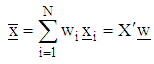 where,
 is an
is an  design matrix and
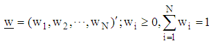 is the vector of weights associated with the design points.The optimal starting point
  is obtained by minimizing the norm
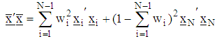 To minimize
  with respect to
  we solve
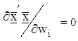 The optimal starting point of search is
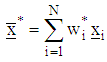
2.2. The Direction of Search
- The direction of search is in the direction of minimum variance and is computed as
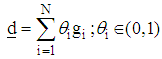 where
where  is the gradient vector and
  weighting factor vector.The direction variance is given as
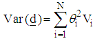 where
where  is the variance of the function at the ith support point. The weighting vector
  is obtained from the partial derivatives
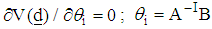 where
where 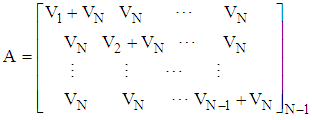
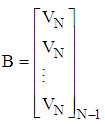 and
and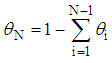 The normalized weighting factor vector
  is given as
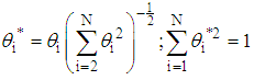
2.3. The Step Length of Search
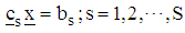
- Given that the response function is constrained and the optimizer lies on the boundary of the feasible region governed by
 The optimal step-length
  of the function
  is obtained as the minimum distance covered in an average step for s number of constraint and is defined as:
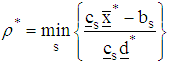 Where
Where  and
and  are vectors and
  is a scalar for s number of constraints, while
  is the optimal starting point and
  is the optimal direction vector.
2.4. The Variance Weighted Gradient Projection (VWGP) Approach
- Let
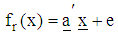 be the n-variate, p-parameter polynomial of degree m, defined on the rth feasible regions
  supported by s constraints. Such that
  where
where  is a p-component vector of known coefficients, independent random variable
  and
and  is the random error component assumed normally and independently distributed with zero mean and constant variance. While
  is a component vector of know coefficients and
  is a scalar for s number of constraints in the rth region.The Variance Weighted Gradient (VWG) method is given by the following sequential steps:i) From
  obtain the design measures
  which are made up of support points from respective regions such that
 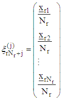 where
where  support points are spread evenly in
  ii) From the support points that make up the design measure compute R starting points as, the arithmetic mean vectors.
 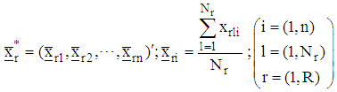 iii) Obtain the n-component gradient function for the rth region.
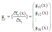 where
where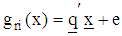 is an
is an  degree polynomial;
 is a t-component vector of known coefficients iv) Compute the corresponding r gradient vectors, by substituting each design point defined on the rth region to the gradient function
  as
as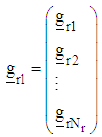 v) Using the gradient function and design measures obtain the corresponding design matrices
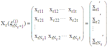 In order to form the design matrix
  a single polynomial that combines the respective gradient function
  associated with each response function
  is
is  vi) Compute the variances of each l design point
  defined on the rth region as
 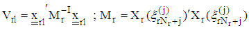 vii) Obtain the direction vector in the rth region as
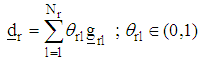 and the normalize direction vector
 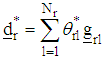 such that
  viii) Compute the step-length
  as
as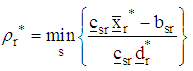 with
with  and
and  make a move to
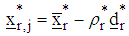 using
using  evaluate the projection operator
  as
as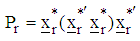 and obtain the projector optimizers for each region
  as
as 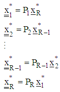 ix) To make a next move set
  and define the design measure as
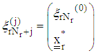 and repeat the process from step (ii) then obtain
 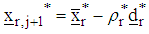 x) If
x) If 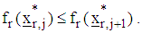 where
where  is the rth feasible region at the jth step and
 is the rth feasible region at the next j+1th step.then set the optimizers as
  and STOP. Else, set
  and repeat the process from (ii).Theorem Let the direction vector
  the weighting factor vector
  is inversely proportional to the variance vector of the function
  where
where 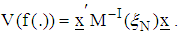 Proof: (By induction)
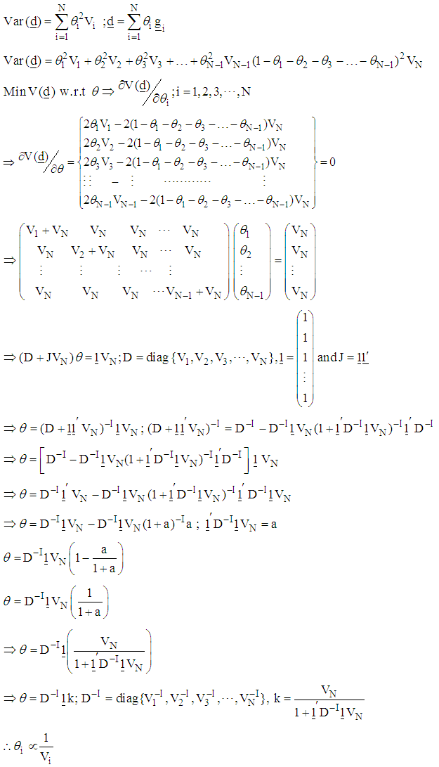
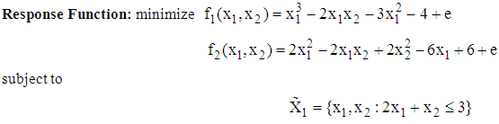
3. Results
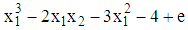
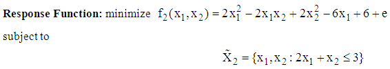
- We present the working of the algorithm using a numerical illustration involving two response functions. The problem is;
 and
and The design regions are defined by
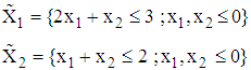 To solve this problem using the VWGP technique, we select design points from
  to make up the respective initial design measures as
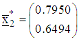
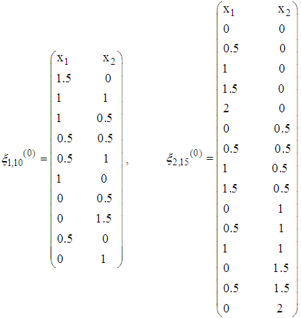 Taking the weighted averages, the initial starting points for the two functions are, respectively,
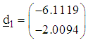
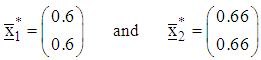 The gradient vectors are obtained as
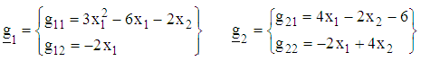 Hence the gradient functions are, respectively,
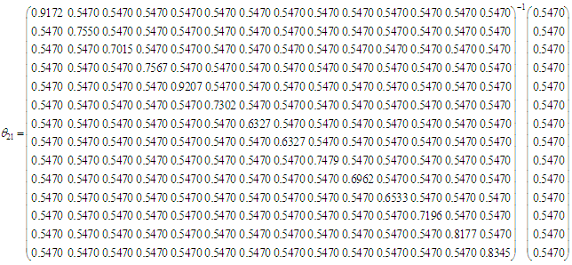
  Using the gradient functions and the design measures, we form the corresponding design matrices as
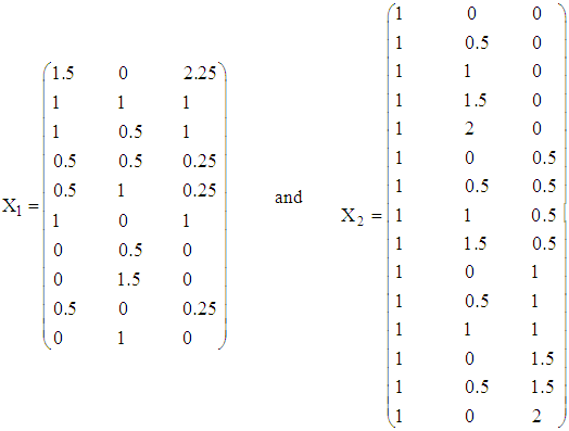 The variances associated with the design points of each design measure are computed as illustrated below for the design point
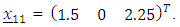 The variance of
  denoted
  is computed as
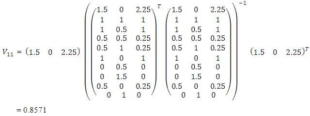 The process continues similarly in obtaining the variance of each design point from the two regions. Thus the vectors of variances are respectively,
 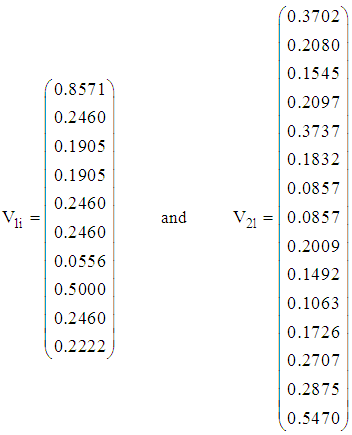 The weighting factors are obtained as
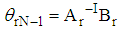 where
where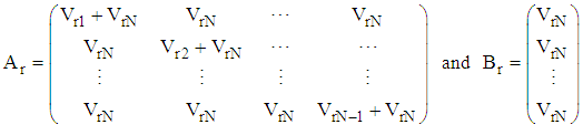 Thus
Thus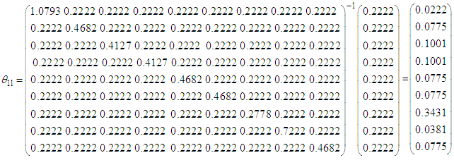 and
and 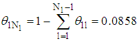
 is normalized as
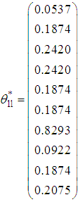
 Thus
Thus  and
and 
 is normalized as
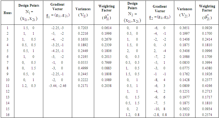
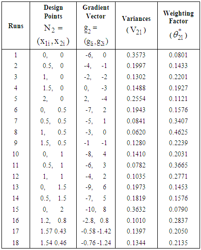
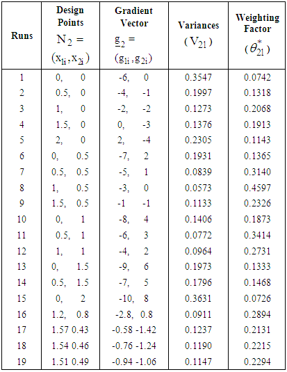
 The computed statistics are summarized in Table 1.
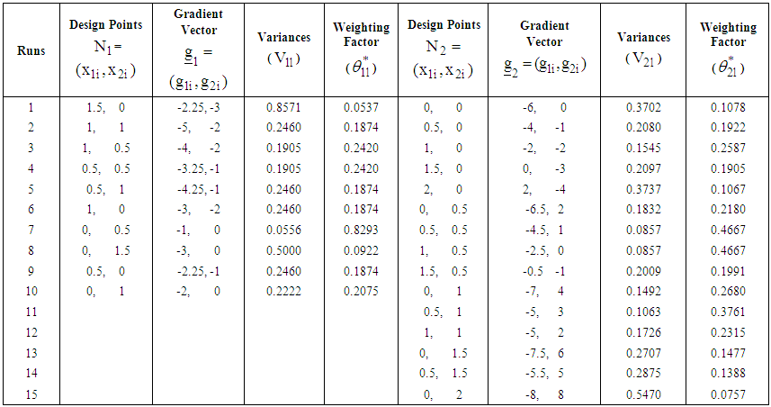 | Table 1. Summary statistics for the first and second response functions at respective design points in the first iteration |
 and
and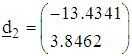 The normalized direction vectors are respectively
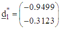 and
and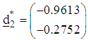 The associated step-lengths are computed as
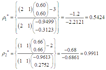 With the starting points of search, the directions of search and the step-lengths we make a first move for each of the functions to
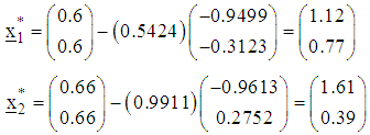
 | Table 2. Summary statistics for the two response functions at respective design points in the second iteration |
 and
and  In order to make a second move, a projector operator
  is formulated by projecting design points from one design space or feasible regions to another feasible region. The resulting projector operator
  is used to compute the projector optimizers
  and
and  which are added to the design measure of respective response function and the process of search continues. The computations are as follows:
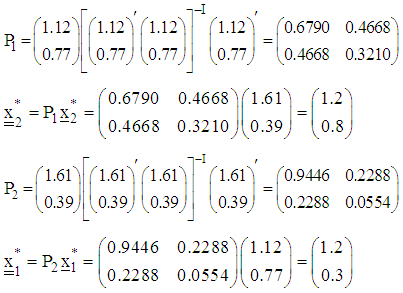 Adding the projector optimizers to the initial design measures result in the following augmented design measures
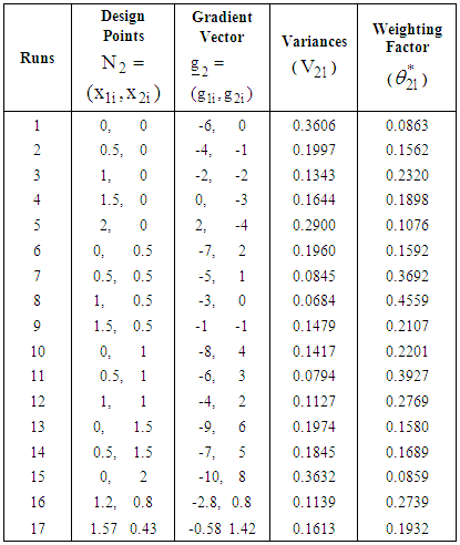
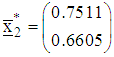
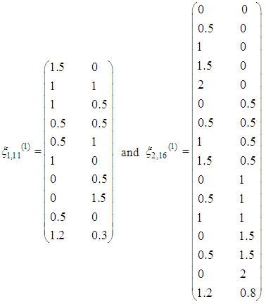 With the new design measures, the computed statistics are summarized in Table 2.The starting points of search at the second iteration are respectively
 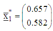 and
and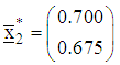 As previously described, the directions of search and the step-lengths of search at the second iteration are computed similarly as
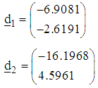 and normalized as
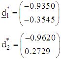 Compute the step-lengths of search are respectively
 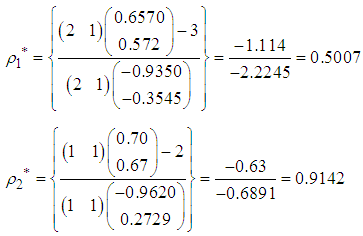 The points reached at the second iteration are respectively
 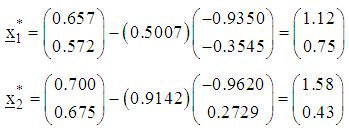 The corresponding values of objective functions are respectively
  and
and  Since for the first function,
 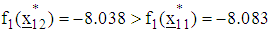 , convergence is established for the first function. However, since for the second function
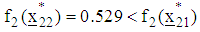
 a next iteration is required. Using a projector operator, a new design point
  is obtained and thus the design measure is augmented as
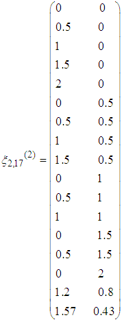 Continuing the process, the computed statistics using the new design measure are summarized in Table 3.
|
 The direction of search, normalized direction of search and step-length of search at the third iteration are respectively
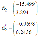 and
and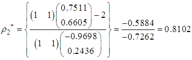 The point reached at the third iteration is
 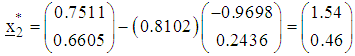 The corresponding value of objective function is
  Since
Since 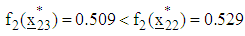 , a next iteration is required. Using a projector operator, a new design point
  is obtained and thus the design measure is augmented as
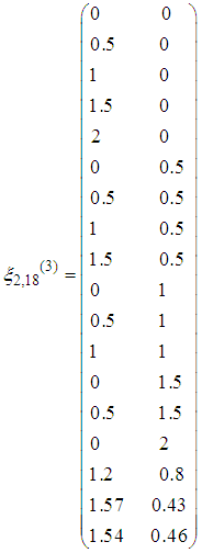 The computed statistics using the new design measure are summarized in Table 4.
|
 The direction of search, normalized direction of search and step-length of search at the fourth iteration are respectively
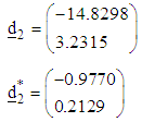 and
and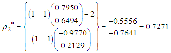 The point reached at the fourth iteration is
 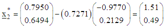 The corresponding value of objective function is
  Since
Since 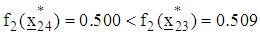 , a next iteration is required. Using a projector operator, a new design point
  is obtained and thus the design measure is augmented as
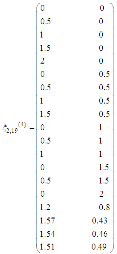 The computed statistics using the new design measure are summarized in Table 5.The starting point of search at the fifth iteration is
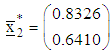 The direction of search, normalized direction of search and step-length of search at the fifth iteration are respectively
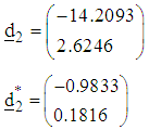 and
and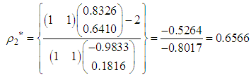 The point reached at the fifth iteration is
 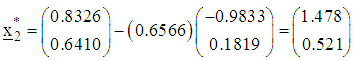 The corresponding value of objective function is
  Since
Since 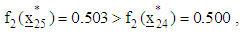 convergence is established and hence no indication for a further search.
|
4. Discussion
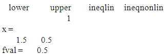
- Variance is a principle commonly used in statistical theories. It has been used in design constructions as well as in optimization problems. Variances of direction vectors have been studied and it is well established that a good direction of search should satisfy the minimum variance property. In optimization, moving in the direction of minimum variance has been shown to optimize performance. This has been clearly stated and proved in literature. Available literatures also show advantage of moving in the direction of minimum variance. The use of variance principle in the VWGP algorithm employed in solving multi-objective problems has assisted in getting optimal solutions with possible minimum iterative moves. Also, optimal choices on the starting point of search and the step-length of search greatly enhanced performance. As mentioned in the literature review, various gradient and non-gradient based optimization methods have been formulated to obtain optimal solutions for constrained polynomial response functions defined over continuous variables. We have compared the solutions obtained using the new algorithm with those obtained using the Quasi-Newton method. With the Quasi-Newton method, results show that the function

 converged after four iterations with optimal values as
 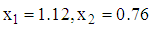 and a corresponding value of response function,
  . Also using the Quasi-Newton method, the function
  converged after four iterations with optimal values as
 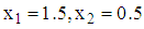 and a corresponding value of response function,
  We observed that the guess initial point requirement of the Quasi-Newton method poses limitation in the use of the Quasi-Newton method. It is sometimes difficult to get a good guess point and thus results in slow convergence of the algorithm or even non-convergence of the algorithm. For the illustration presented in this paper, the optimal solution for the first function was found at the first iterative move and the optimal solution for the second function was found at the fourth iterative move. The printout from MATLAB showing the results are presented in Appendices A and B.The use of the Variance Weighted Gradient Projection (VWGP) method is a reliable optimization method for optimizing polynomial response surfaces defined by constraints on different feasible regions. The algorithm is reliable and converges to the desired optima with few iterative steps. The performance of the new algorithm agrees with the suggestion of [7] that a good algorithm should have less computation and a quick convergence. The present study may be extended to searching for optimal solutions to multi-objective functions defined on distinct regions but where some or all of the regions may have two or more objective functions.
5. Limitation of the Method
- The VWGP algorithm is not yet implemented in a Mathematical or Statistical software and hence the computation time and memory resources are not addressed.
ACKNOWLEDGEMENTS
- We sincerely wish to acknowledge the assistance and useful contributions of Professor I. B Onukogu of the Department of Mathematics and Statistics, University of Uyo, Nigeria.
Appendix 1
- The Quasi-Newton Optimization with the aid of MATLAB
 QN%%%%%%%%%%%%%%%%%%%%%%%%%%%%%%%%%%%%%%%%%%%%%%%%%%%%%%%% %%%Diagnostic Information Number of variables: 2
 Algorithm selectedmedium-scale%%%%%%%%%%%%%%%%%%%%%%%%%%%%%%%%%%%%%%%%%%%%%%%%%%%%%%%%End diagnostic information
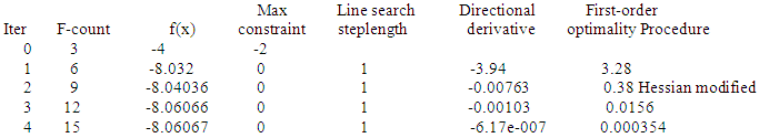 Optimization terminated: magnitude of directional derivative in search direction less than 2*options.TolFun and maximum constraint violation is less than options.TolCon.Active inequalities (to within options.TolCon = 1e-006):
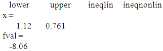
Appendix 2
- The Quasi-Newton Optimization with the aid of MATLAB
 QN%%%%%%%%%%%%%%%%%%%%%%%%%%%%%%%%%%%%%%%%%%%%%%%%%%%%%%%%Diagnostic Information Number of variables: 2
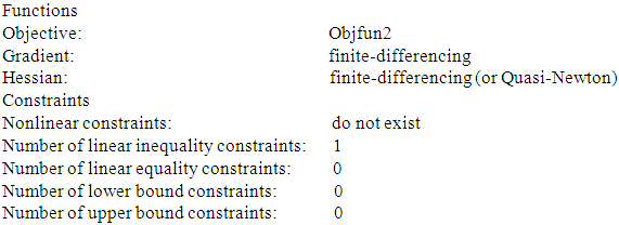 Algorithm selectedmedium-scale%%%%%%%%%%%%%%%%%%%%%%%%%%%%%%%%%%%%%%%%%%%%%%%%%%%%%%%% %%%End diagnostic information
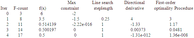 Optimization terminated: first-order optimality measure less than options.TolFun and maximum constraint violation is less than options.TolCon.Active inequalities (to within options.TolCon = 1e-006):