1. Introduction

The measurements obtained by propagating seismic wave through the subsurface in which the earth’s subsurface properties derive from seismic waves reflection can be measured is known as seismic data. Seismic data however is a reflector of constitutes of different layer in the formation of rocks or different rock formations as layers of reflectors. Seismic data is also known as an image of the earth subsurface and can also be considered as different rock type, the fluids in the rocks which cause seismic reflection events and the geological features of the earth subsurface can be gotten by explorationist through seismic data. For details and a review of seismology, see [1-4].

Seismic studies are a key stage in the search for large scale underground features such as water reserves, gas pockets, or oil fields [5]. Sound waves, generated on the earth’s surface, travel through the ground before being partially reflected at interfaces between regions with high contrast in acoustic properties such as between liquid and solid. Seismic method is the generation of sound waves of low frequency at the earth surface by high energy source [6]. They reflect back when encountering different layers of rock where the properties of rock changes as they travel down the earth and is recorded by the receivers as set of field data, interpreted by a geophysicist when processed in a computer center. Reflector’s depth is known when the time taken for the sound wave from explosive move to the reflections interface (rock properties) and returned to the reflecting interface is known and the differences within the reflecting interface in the subsurface rock properties is known by the magnitude of the reflected energy signal. Initially, acquisition of seismic data was done along straight lines (2D); the data needed to make a map were obtained through shooting some lines across survey area [7, 9]. The acquired data will then be used for analyzing velocity and density for the volume of oil deposited in a particular location (prospect), analyzing these data possess a lot of problem for researchers because of its complexity. Literature to the best of our knowledge show that among various methods of analyzing this data are despiking, kriging, and fourier transform. Multiple problems, including high computational cost, spurious local minima, and solutions, have prevented widespread application of these methods. These problems are fundamentally related to a large number of model parameters and to the absence of low frequencies in recorded seismograms [8, 9, 11]. Geostatisticians are therefore confronted with a multitude of problems when trying to analyse seismic data to produce a model of the subsurface that can help identify where oil and gas is deposited, or assist reservoir engineers to optimise the production of a field. The sheer volume of a seismic data set is itself a barrier to interpretation and this imposes a basic limit based on the computing power available and the speed of the algorithms used to process the data. In this paper, we proposed a spline function model to solve this problem.

Spline functions have proved to be very useful in numerical analysis, in numerical treatment of differential, integral and partial differential equations, in statistics, and have found applications in science, engineering, economics, biology, medicine, etc. Spline interpolation is a form of interpolation where the interpolant is a special type of piecewise polynomial called spline. Spline interpolation is often preferred over polynomial interpolation because the interpolation error can be made small even when using low degree polynomials for the spline [10]. Spline interpolation avoids the problem of Runge’s phenomenon, in which oscillation occurs between points when interpolating using high degree polynomials [12, 13, 15, 16]. Cubic Spline interpolation is a special case of spline interpolation that is used very often to avoid the problem of Runge’s phenomenon. This method gives an interpolating polynomial that is smoother and has smaller error than other interpolating polynomials such as Lagrange polynomial and Newton polynomial [16, 17].

The rest of the paper is organized as follows. In Section 2, the theory of spline function is presented leading to developing spline function model for the seismic dataset. This is followed by the method of data analysis which is in Section 3 while in Section 4, numerical illustration will be carried out. Finally, there is a conclusions’ section followed by references.

2. The Theory of Spline Function

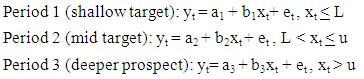
The process of combining different polynomials together at joined points is used in producing spline function. That is, the interval between the lower limit (R₁) and the upper limit (R₂) is splited such that a curve can be approximated into (P+1) sub-intervals divided by joined points (p) which is inner boundaries. We examine a situation where two sub-intervals is formed by splitting one interval (L₁, L₂) with only a joined point. In any interval, there is spline function and a stated ‘m’ dimension maximum term describing the polynomial conversely, sequence (digit of coefficient describing the polynomial, and it is one plus the dimension). If we consider ‘p’ as the polynomial sequence where the dimension will be ‘p+1’. These two polynomials would be expected to become united with uniform consistency in the inner joined points (k₁). For a simple situation which shows that derivatives is equivalent to the sequence which the dimension is one greater. Equivalent polynomial would exist in a situation where the two polynomials are the same with the derivative where sequence and dimension are equivalent [16, 18]. The polynomial ranging up to the full interval contains one degree of freedom less than the spline function represented. For illustration, if a linear line section which is a polynomial of one degree with the same derivatives equal to dimension ‘o’ after connected at knot, in a nutshell, they contain the same values at the breakpoint and they also commonly connect. In view of first polynomial having two degree of freedom (gradient as well as intercept), while the second polynomial contain a single degree of freedom (gradient) with the knot earlier used in determining its value, the entire polygonal line consist of three dimensions of freedom [19, 20]. For example, the relationship between depth of explosives and the seismic velocity over an acquisition time that involves shallow target, mid target and deeper prospect on the data is considered. The data is grouped into three different subsets as well as three estimated time trends.

The following model is postulated by considering a linear time trends:-

When (L,u) is the time interval. The estimated trends can be represented in the figure (1) below:

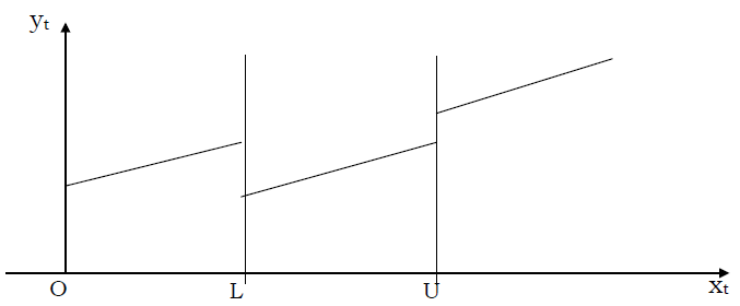Figure 1. Trends Estimated (Discontinuity at Joined Points)

There are discontinuities at the joined points t=L and t=U considering the function in the unrestricted estimation process. One method of overcoming this is to reformulate the model by defining;

Function is reparamaterized as: y_{t =} k_o + k₁ P_1t + k₂ P₂t + k₃P_3t+ e_t

The parameters which meet at the joined points can be estimated by using ordinary least squares method.

3. Methodology

The method proposed here takes as its starting point by considering smoothing to remove the effects of noise, before moving on to identify key features within the data using least squares method. This will lead us to the selection of the best model using spline functions. We considered the relationship between depth of explosives and the seismic velocity over an acquisition time that involves shallow target, mid target and deeper prospect on the data. The data is grouped into three different subsets as well as three estimated time trends: The following model is postulated by considering a linear time trends:

When (L,U) is the time interval.

Function is reparamaterized as: y_{t =} k_o + k₁ P_1t + k₂ P_2t + k₃P_3t + e_t

Notations

T = Time of recording the data in mini-seconds

X_t = Depth of the explosive (source) in metres

y_t = Velocity obtained after the detornation of explosives

T₁ –T₁₅ = Time for the shallow target in mini-seconds

T₁₆-T₂₅ = Time for the mid target in mini-seconds

T₂₆-T₄₀ = Time for the deeper prospect in mini-seconds

K₀ = Replacement velocity (ms^-1)

K₁ = Reciprocal of time at shallow target

K₂ = Reciprocal of time at mid target

K₃ = Reciprocal of time at the deeper prospect

P_1t = Depth of signal at shallow target (m)

P_2t = Depth of signal at mid target (m)

P_3t = Depth of signal at deeper prospect (m)

The natural question is how should we choose the “interpolating points” from such seismic data so as to construct the desired smoothing function. Normally, these points are extracted from the data, in a regular fashion or manually selected.

4. Numerical Application

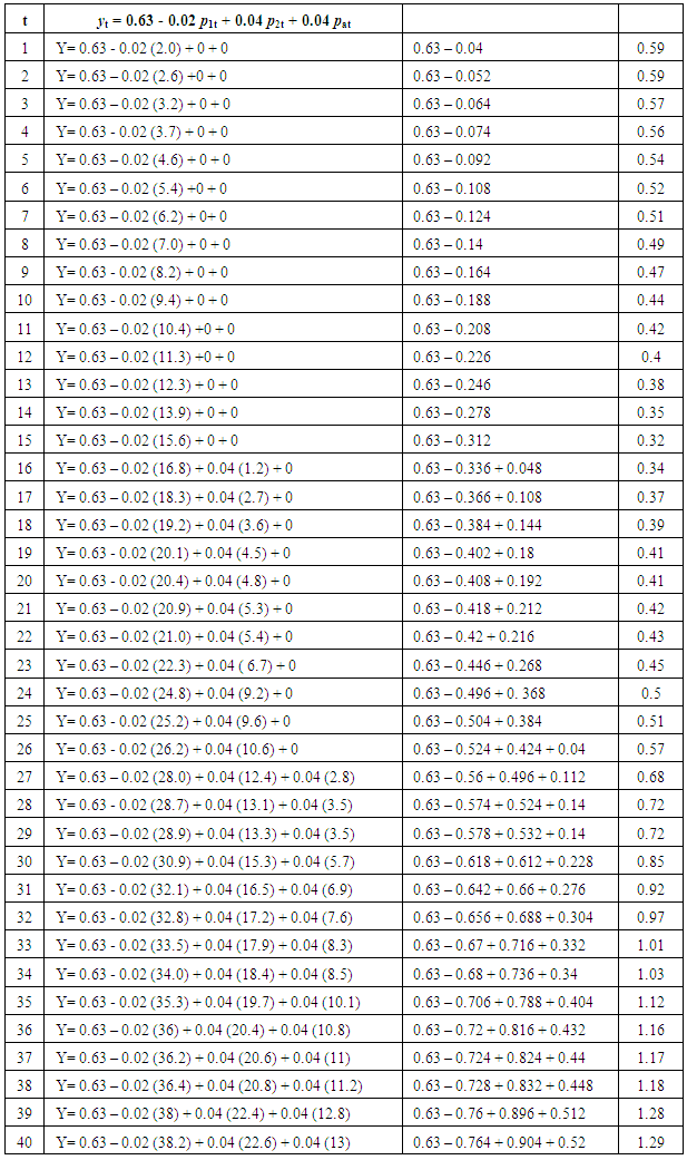
We now illustrate the application of the proposed method to some common practical situations. We start by testing the ability of the method to smooth a sequence of the three periods. The following table shows the depth of explosives (x_t) in metres and velocity (y_t) in (1000ms^-1) for a data of 40000msec.

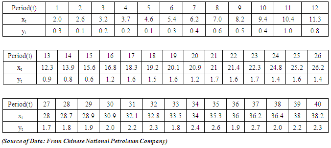We classify the data into the following arbitrary period:

Period 1 (t₁ + t₁₅), Period 2 (t₁₆ – t₂₅) Period 3 (t₂₆ – t₄₀) We define the following

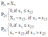The new set of data is now the following:

Table 1. The new set of data

We consider now the linear spline function:

y_t = k₀ + k₁ p_1t + k₂ p_2t + k₃ p_3t + e_t.

The model can now be fitted by the usual least squares method to estimate the parameters k₀, k₁, k₂ and k₃ respectively: The fitted parameter estimates is shown in the table below

Table 2. Summary table of the fitted parameter estimates

Thus reparameterize the function as

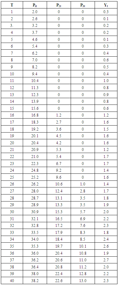
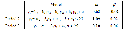
From the above parameters, we can obtain the linear spline function as:

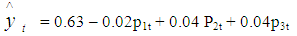Fitting the data into the Estimated Model

Table 3. Fitted data based on the estimated model

5. Discussion

From the graph in Fig 2.1, we can deduce that if the velocity is plotted against the depth using the observed data, (that is, without the application of the proposed model). Velocity reversal is seen at the following depth intervals, 20m to 27m and 33m to 37m, whereas after fitting the same data into the proposed model, the velocity reversal at those depth intervals have been resolved as seen in Fig 2.2 and the velocity now has a common trend which signifies increased with depth which can now be used for migration and pore pressure prediction. The proposed model has help in the smoothing of the velocity (that is, attenuation of noise or elimination of unwanted signals (outliers). The velocity reversal seen in the predicted model which is between the depth intervals 0 to 15.5m is as a result of unconsolidated layer in the near surface which also signifies zone of unreliable velocity, but the proposed model has helped in fitting a correct velocity by redefining the outliers. The proposed model also helps in predicting where to place floating datum which is the velocity field at the depth where it begins to increase or the velocity field that shows the difference between unconsolidated layer and consolidated layer. The velocity field at this datum will be used to correct for refraction statics. The most important factor when dealing with real data like seismic data is to choose a suitable parameter of smoothing. The results of calculation for small values of this parameter heavily depend on the measurement error, so the resulting velocity graph gets a sawtooth form. If the smoothing parameter is too large, then oversmoothing of initial data occurs. It leads to losing data informativeness. Therefore, the velocity graph becomes too smooth and far from the truth.

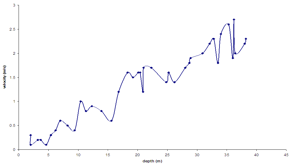Figure 2.1. Velocity versus depth before the model

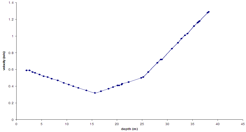Figure 2.2. Velocity versus depth after the model

6. Conclusions

In this paper, we considered developing a model that will help in seismic data analysis such as interpolation, smoothing and noise reduction. Spline function is functional to a wider range of problems which are formulated basically in a non discrete structure relatively to the discrete structure. Computational tasks such as the search for extreme differentiation and integration are uncomplicated in altered spline field and carried out in this respect. Some of the applications involved approximation of higher categorizes derivatives in contaminated data and border discovery in reflection processing. The spline coefficients are achieved by method of alteration linearly, which is different from other frequently transformed methods (trigonometric functions, Fourier, etc.), and can also be executed professionally when filtering linearly. The approach proposed here is based on simple statistical procedures which aim at smoothing out noise and using contextual information to identify coherent horizons. In particular, smoothing splines are used to smooth seismic data by explicitly evaluating their transform functions for splines of any order. It appears also that greater smoothing can be applied to the traces, without overwhelming the major features, than would be the case if the aim was to estimate the signal.