Akpan N. P.1, Bassey N. A.2
1Department of Mathematics and Statistics, University of Port Harcourt, Nigeria
2Department of Statistics, Akwa Ibom State college of Art and Science, Nung Ukim, Nigeria
Correspondence to: Akpan N. P., Department of Mathematics and Statistics, University of Port Harcourt, Nigeria.
| Email: |  |
Copyright © 2017 Scientific & Academic Publishing. All Rights Reserved.
This work is licensed under the Creative Commons Attribution International License (CC BY).
http://creativecommons.org/licenses/by/4.0/

Abstract
One of the reasons pregnant women has complications during pregnancy or child delivery is negligence of antenatal appointments and inability to adhere to medical advice. Due to the inconsistencies on the antenatal appointments, data generated from it has not been frequently used for statistical analysis. In this study, the application of survival analysis on antenatal appointment data was a priority. The survivorship function of the data was estimated using Kaplan-Meier method. The results showed that pregnant women attend the antenatal care for an average period of six (6) months. Cumulative hazard curves were plotted and they revealed that the antenatal appointment data can best be analyzed using the Weibull survival function and Weibull hazard function with parameters α = 2.89 and λ = 0.004.
Keywords:
Survival analysis, Antenatal appointment, Kaplan-Meier method
Cite this paper: Akpan N. P., Bassey N. A., Application of Survival Analysis on Antenatal Appointment, International Journal of Statistics and Applications, Vol. 7 No. 1, 2017, pp. 12-17. doi: 10.5923/j.statistics.20170701.02.
1. Introduction
Survival analysis is a specialized field of mathematical statistics developed to study a special type of random variable of positive values with censored observations of which survival time events are the most common (Ma and Krings 2008). The main variable of interest is time – to – event. Examples of time – to- event random variables are incubation time of disease such as AIDS, failure time of certain machine components, times to death of patients with certain disease, the length of time of economic recessions and the occurrence of the next traffic accident. Other kinds of events which could be studied by survival analysis are divorce, criminal recidivism, child bearing, unemployment and graduation from school (John Fox, 2014). Initially, survival analysis was useful only in the field of biostatistics and was mainly applied in medical researches for better analysis of life table data. It was also used to study death as an event specific to medical studies and demographic studies (Narendranathan et. al. 1993). As from 1970 till date, the statistical technique have been frequently applied in several fields of human endeavour such as engineering, economics, social sciences, medicine and public health just to mention but few. Its name varies from discipline to discipline, in engineering, it is called failure time analysis, in sociology it is referred to as history analysis. It is called survival analysis in biostatistics and medicine. The advantage of survival analysis is its ability to handle censoring in an effective manner (Ma and Krings, 2008) although observation of censoring or incomplete information are not necessary for the application of survival analysis.
2. Materials and Methods
The data used in this study were obtained from the record unit of Poly clinic, Ini Local Government Area of Akwa Ibom State, Nigeria. The data set consisted of 1311 pregnant women who visited the clinic for booking and antenatal appointment between the year 2009 to 2013. There are several models used in survival analysis. Naturally any distribution of non-negative random variables could be used to describe durations. In this study, we are interested in parametric models such as the Exponential models, Weibull model and Gompertz models. This is because they have closed forms expressions for survival and hazard functions. Survival function s(t):This represents the probability that an individual survives from the time origin to some time beyond t. It is given by | (1) |
Hazard function λ(t):This is the probability that an individual stops attending antenatal care at time t, given that she had survived up to that time. It is linked to the probability density function and survival function as follows: | (2) |
Kaplan – Meier Estimator:Suppose the events of interest occur at time t1 < t2 < ----< ti < --------- < tn, then the Kaplan Meier estimate of the survival function is given by;  | (3) |
where ni is the number of pregnant women who continue their antenatal care at time ti. di is the number of those who stopped their antenatal care at time ti. Exponential DistributionThe exponential distribution model (t~exp(λ)) is the simplest model and assumed a constant risk over time. The probability to event of interest within a particular time interval depends only on the length but does not depend on the location of the interval.  The parameter λ attains only positive values, and the following formula are associated with the distribution.
  | (4) |
 | (5) |
 | (6) |
 | (7) |
Weibull Distribution:The Weibull model is a generalization of the exponential model with parameters α and λ which are called shape and scale parameters respectively. The parameters determine the shape and scale of the hazard function. The convenience of the Weibull model for empirical work arises from the flexibility and simplicity of the hazard and survival function. Its functions are as follows: | (8) |
 | (9) |
 | (10) |
 | (11) |
Gompartz Distribution:A random variable follows a Gompertz distribution with parameters a>0 and b>0 (t ~ Gompertz (a,b) ) if the following relations hold: | (12) |
 | (13) |
 | (14) |
 | (15) |
Plots for Parametric Models:In order to investigate the appropriate parametric model that can be used for the analysis of the antenatal care data, we used a straight line fit. We used the cumulative hazard Λ(t) which is a better determinant of the appropriate survival distribution because its form is more distinct than that of density function f(t) or the survival function s(t), (Gross and Clark, 1975).Bradburn et.al (2003) stated that; i. The plots of log Λ(t) against t is linear for exponential distribution.ii. The plots of log Λ(t) against log t is linear for Weibull distribution.iii. The plots of log Λ(t) against t is linear for Gompertz distribution.Therefore, we plotted the graphs in order to obtain the suitable model and the survival function was used to estimate the cumulative hazard function thus; | (16) |
In plotting log Λ(t) against log t, if the line is approximately straight then its slope gives an estimate of the shape parameter (α) while the exponential of the intercept gives an estimate of the scale parameter (λ) of the Weibull distribution. Also, if the slope of the line is approximately unity (1), then the exponential model is considered appropriate. (Collett D, 1994).In order to estimate the median survival time, we draw a horizontal line from the vertical axis to the curve at Ŝ(t) = 0.5, the point of intersection with the curve determines the median. The mean survival time based on the Kaplan – Meier product limit is obtained by; | (17) |
3. Analysis/Discussion
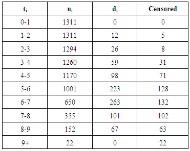
ABBREVIATIONS: Table 1. The Antenatal Data
 |
| |
|
ti -Survival period in months ni-Number of pregnant women who were able to continue their antenatal appointment for the period ti.di-Number of pregnant women who were unable to continue their appointment.Censored - Number of pregnant women who delivered in the period ti. From equation (3), the unconditional probability that a pregnant woman will continue her antenatal appointment beyond any time ti is estimated as follows: 
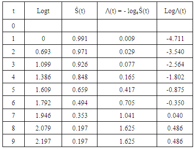
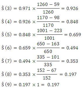 Table 2 for plotted values.
Table 2. Plotting for Exponential Distribution
 |
| |
|
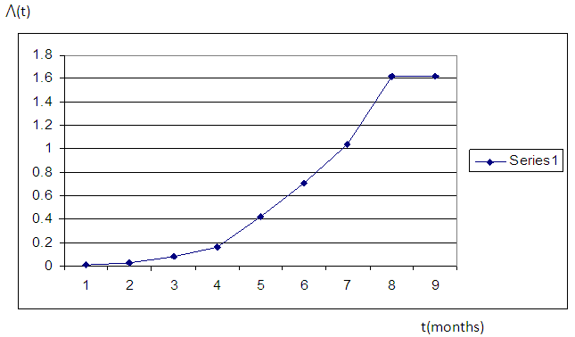 | Figure 1 |
Plotting for Weibull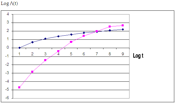 | Figure 2 |
Plotting for Gompartz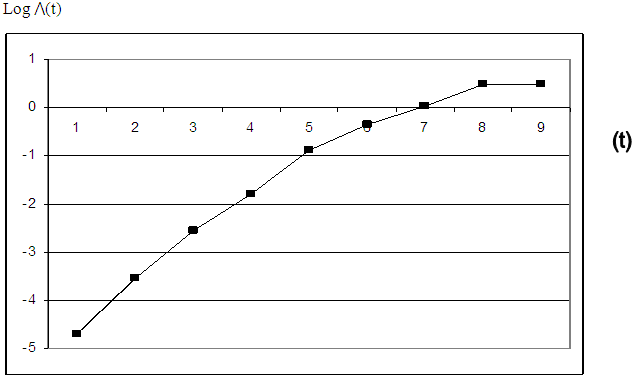 | Figure 3 |
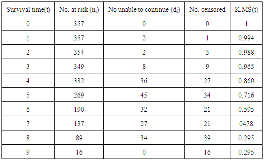
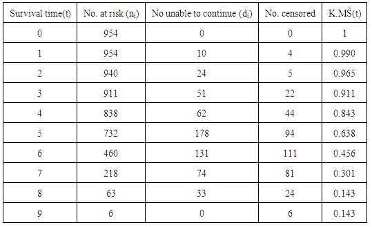
From the graphs, the plots of cumulative hazard (Λ(t)) against time (t) and the plots of logarithm of cumulative hazard, logΛ(t) against time (t) are not linear, but the plot of logarithm of cumulative hazard, log⋀(t) against logarithm of time, log(t) is linear which implies that the ante-natal data can be modeled by using Weilbull survival distribution with shape parameter (α = 2.89) and scale parameter (λ = 0.004).Therefore, the antenatal data can be modeled as:(i) Pdf: f(t) = 2.89 λt2.89-1 e-λt^2.89(ii) Survival function: S(t) = e-λt^2.89(iii) Hazard function: λ(t) = 2.89 λt2.89-1(iv) Cum. Hazard function: Λ(t) = λt2.89 Where λ = 0.004The estimated mean survival time for the antenatal data is:μ = 1.0(1) + (0.991) (2-1) + (0.971) (3-2) + (0.926)(4-3) + (0.848)(5-4) + (0.659)(6-5) + (0.494)(7-6) + (0.353)(8-7) + (0.197)(9-8) = 6.439 = 6 monthsMean survival time for teenager:µ = 1.0(1)+0.994+0.988+0.965+0.860+0.716+0.595+0.478+0.295= 6.891Mean survival time for adults:µ = 1.0 (1)+0.990+0.965+0.911+0.843+0.638+0.456+0.301+0.143 = 6.247The mean survival time for teenager is 6.891 (i.e approximately 7 months) while that of the adult is 6.247 (i.e approximately 6 months).From figure 4, the median survival times for the teenager group and adult group are 7 months and 6 months respectively, while the median survival time for the entire pregnant women is 6 months as shown in figure 5.Table 3. Kaplan Meier Estimates for teenager (age<20 yrs)
 |
| |
|
Table 4. Kaplan Meier Estimates for adults (Age≥20)
 |
| |
|
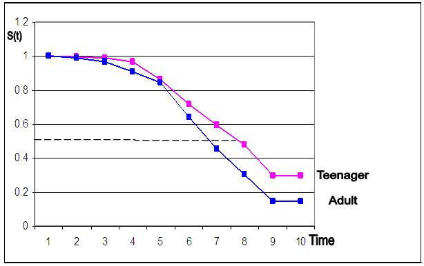 | Figure 4. Kaplan Meier Curves for Teenager and Adult |
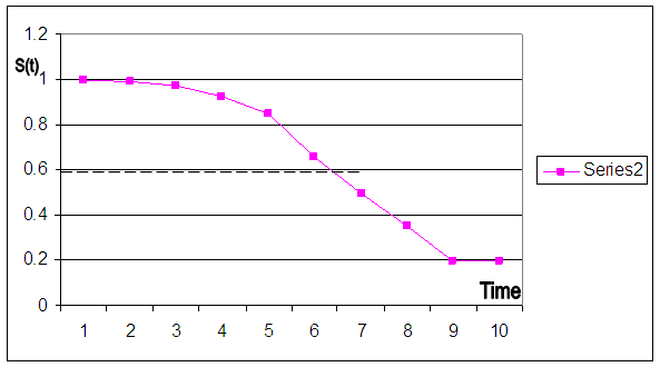 | Figure 5. Kaplan Meier curves for Antenatal Data |
4. Conclusions
From the result we concluded that the probability that pregnant women will continue their antenatal care reduces with time. Moreover, the mean and median survival time being equal to 6 reveals that pregnant women attend their antenatal care six times on average. From the results we also concluded that the antenatal appointment data can best be analyzed parametrically using the Weibull function.The probability of a pregnant woman attending the antenatal care for time (t) can be modeled as S(t) = e-λt^α The probability that a pregnant woman will stop attending the antenatal care after time t can be modeled as: Where λ = 0.004 and α = 2.89.
References
| [1] | Bradburn, M. J. et, al (2003). Survival analysis part 1: basic concepts and first analyses. British Journal of cancer 89(2): 232-238. |
| [2] | Collett, D (1994). Modeling survival Data in medical Research. London: Chapman & Hall. |
| [3] | Gross, A. J. and Clark, V. A (1975). Survival Distributions: Reliability Applications in the Biomedical Sciences. John Willey & Sons New York. |
| [4] | John Fox (2014). Introduction to Survival Analysis. Lecture notes (online). http://socserv.mcmaster.ca/for/courses/soc761/survival analysis. pdf. |
| [5] | Ma, Z. and Krings A. W (2008). Survival Analysis Approach To Reliability, Survivability and Prognostics and Health Management. The 2008 IEEE-AIAA Aerospace Conference, Montana, March 1-8, 2008. |
| [6] | Narendranathan et. al. (1993). Modeling the Probability of Leaving Unemployment: competing risks models with flexible baseline hazards. Journal of the Royal Statistical Society, series c, Applied statistics, 42 (1), pp. 63-83. |


 The parameter λ attains only positive values, and the following formula are associated with the distribution.


 Table 2 for plotted values.


 Where λ = 0.004 and α = 2.89.
 Abstract
 Reference
 Full-Text PDF
 Full-text HTML