1. Introduction

There are more than one thousand financial companies in Nigeria offering a wide variety option to investors. Given this wide of choice and increasing bad publicity around failed investment companies, financial advisors are facing a daunting task of prudently investing their client’s hard earn money. Thus, models of insolvency prediction that help identify future business failures or financial distress is important tools for advisors. The model may not specifically tell the manager what is wrong, but it should encourage them to identify problems actions to minimize the incidence of failure. A predictor model may warn an auditor of company vulnerability and help protect them against charge of neglect of duties in not disclosing the possibility of insolvency.

In this research, “failure” is define as a registered company being liquidated. One of the most significant threats for many businesses today despite their size and the nature of their operations is insolvency. Between 2008 and 2009, large numbers of financial institution failed over the world with devastating economy, social and political consequences. In Nigeria, almost half of the banks have one of distress or the other.

Leading causes of corporate failure can be into economic, financial neglect, fraud or disaster (Anderson, 2006) Economic factors including industrial weakness and poor location while financial factors include excessive debt and cash flow problems. One widely accepted method of assessing financial statement is ratio analysis which uses data from the balance sheet and income statement to produce values that have easily interpreted financial meanings. The financial statement analysis and financial ratio believe to have originated in the United States (Horrigan, 2001). The major development that create data are the emergence of the corporation as main organizational form of business enterprise, resulting in the separation of management from ownership and the fast increasing role of financial institution (e.g. banks, investment and insurance companies) as the major suppliers of capital for business expansion requiring formal evaluation of borrowers, credit worthiness, consequently analyzing corporate financial data.

The objectives of this study include:

a. To construct a neural network for predicting companies’ insolvency and to compare its forecasting capability to that of parametric models.

b. To test the reliability of ratio analysis and the application of multiple discriminant analysis.

c. To use neural network as a tool for predicting insolvency in the Nigerian financial institutions.

The financial service industry in general and the foreign exchange market in particular were severely affected over the years by the unstable environment created by the high and accelerating inflation rapidly growing liquidity, sharply rising market interest rates and the political environment under these condition, financial weak institution proved unable to cope and the ensuring wave of default eroded confidence in the banking sector.

According to Agenor et al (2004) an excess liquidity demand function of the excess reserves requirement was a function where bank’s holding of excess liquidity over and above requirement was a function of the excess reserved to deposits lagged by one year. Using patterns of excess liquidity in sub-Saharan Africa, Saxegaard (2006) extended Agenor et al (2004) model by proposing a framework for how a decomposition of excess liquidity can be achieved. Bordo et al (2001) also asserts that crises are an intrinsic part of business cycles and results from shocks to economic fundamentals when the economy goes into recession or depression, asset return are expected to fall.

Unegbu and Tasie (2011) tested the efficacy of ‘CPT’ cash flow statement and percentage trend analysis model to identify false financial statement and examined further some relevant literature in an attempt to develop analytical tools for detecting false statement. Henebry (1997) used both cash flow proportional hazard model to test for stability of the model over time. The result indicates that none of the specific formation were stable across different horizon for the same starting date.

Martkanen et al (1991) used a time series approach with transformation analysis to predict financial failure. Theodossious (1993) applied sequential procedure to predict a business tendency towards failure, Kumar and Ganeslingam (2001) applied principal component analysis and cluster analysis to predict the financial distress of major companies.

Amadasu (2012) in his work bank failure prediction showed the ratio retained earning/total assets are most significant in a failing firm, he also found that working/total assets among others should be closely taken care of.

Ibiwoye et al (2012) propose that the insurance industry serves as a medium for fund mobilization. An insolvency prediction model was constructed based on ANN approach which can be used to evaluate the financial capability of insurance companies. Onyeiwu and Alimeke (2012) applied MDA techniques to Nigerian organization to ascertain it ability to effectively discriminate unhealthy organization in Nigeria manufacturing industry. Financial statement was used as instrument for prediction of corporate heath, there was 70% right classification of healthy organization and 80% correct classification of unhealthy organization. Okezie (2011) examined the relationship between capital ratios and bank distress and also compare the efficacy of three ratios as prediction of distress. Ani and Ugbawka (2012) in their study detecting early warning Bank distress signal in Nigerian applied multivariate discriminant analysis model as proposed by Altman in 1968 to group of failed and healthy banks in Nigeria to ascertain if MDA is a veritable tool to predict business failure. The study showed that MDA not only predicts business failure but revealed most important that the warning signals of impending failure become manifested one to two years before the study banks actually failed.

Neophyton et al (2000) developed and validate a failure classification model for UK industrial companies using logit analysis and neural network in predicting corporate failure, the result indicates that a parsimonious model that includes three financial variable can yield an overall correct classification accuracy of 83% one year prior to failure.

Goss and Vozikis (2010) used neural network on a non-parametric model alternative to past techniques and showed how this methodology more effectively predicts insurer insolvency than parametric models. Chung at; al, (2008) in insolvency prediction model using Multivariate Discriminant Analysis and Artificial Neural network for the financial industry in New Zealand utilized MDA and ANN in their study to create an insolvency prediction model that can effectively predict any future o a finance company in New Zealand. The result indicates that the financial ratios of a field company differs significantly from non-failed companies and that failed company were also less profitable and less liquid and had higher leverage ratio and lower quality assets.

2. Methodology

This study uses secondary data and hypothesis testing to assess the relationships in a pattern of financial ratios of failed and non-failed companies. Data were collected from companies that filed for receivership or failed from (1996-2012) extracted from the Nigerian company financial statements over the accounting period of one year 2012. The various corporate financial statements were collected from their respective website/brochures. Overall data were collected from 15 unknown failed companies and 13 non-failed companies. Data was analyzed using the SPSS statistical software package, R consul and C#.

2.1. Multivariate Discriminant Analysis (MDA)

Discriminant analysis is a statistical procedure which allows us to classify cases in separate categories to which they belong on the basis of a set of characteristic independent variables called predictors or discriminant variables. The target variable (the one determining allocation into groups) is a qualitative (nominal or ordinal) one, while the characteristics are measured by quantitative variables.

For each respondent a score is computed using the estimated linear combination of the predictors (the discriminant function), when the discriminant score is standardized to have zero mean and unity variance it is called Z score.

Discriminant analysis characterizes an individual, or a phenomenon, by a vector of variables which constitute a multivariate density function. The discriminant function maps the multidimensional characteristics of the density function of the populations variables into a one-dimensional measure, by forming linear combination (Zavgren 1983). The linear discrimination functions is as follows:

(1)

Where: Z = decriminant score for the company i

X = vector of n independent variable or characteristics

A = vector of discriminant coefficient

MDA computes the discriminant and selects the appropriate weight (cut –off score) which will separate the average values of each group, while minimizing the statistical distance of each observation and its own group means (Altman 1993). By using the Z score and cut-off score, a company is classified into failed or non – failed. The dependent variable is set out as a categorical variable, and independent variable are numerical.

2.2. Artificial Neural Network (ANN)

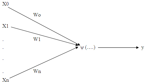
An artificial Neural network is a computer algorithm which can be “trained” to imitate the cellular connections in the human brain (Hwertz, Krogh & Palmer 1991). It consist of a large number of interconnected elementary processing units to compute data. The network’s processing results are derived from the collective behavior of its units and are dependent on how the unit interacts with each other (Altman, Marco & Varetto 1994). By processing and evaluating the interactions in a complex set of prior data, a neural network attempts to assign proper weights to the respective input to allow for correct deduction.

According to Nelson and Illingworth (1990), there are infinitely many ways to organize a neural network although perhaps only two dozens models are in common usage. A neural network organization can be described in terms of its neurodynamics and architecture. Neuridynamics refers to the properties of an individual artificial neuron that consist of the following:

a. Combination of input(s)

b. Production of output(s)

c. Type of transfer (activation) functions; and

d. Weighting schemes, i.e. weight initiation and weight learning algorithm (synapses)

Figure 2.1 presents an artificial perception neuron model with n inputs {x₁, x₂, …., x_n} in which each input x₁ has an associate synapse w_i, and an output y.

Figure 2.1. Artificial perception neuron model

There is also an additional neuron parameter, named w_o, known as bias that can be interpreted as a synapse associated to input x_o = -1. The output of the neuron y is based on the product between input vector x (x_o, x₁, x₂, ……, x_n) and vector w (w_o, w₁, w₂, …, w_n) composed of synapses, including the bias (w_o),

(2)

The neuron output is then obtained through the activation function of neuron y = ψ(x, w), in which a hyperbolic tangent function is usually adopted (sigmoid –nature function), define by a generic value a; however, it is convenient to use other activation functionsin certain scenarios

(3)

the artificial neuron model is feed forward, that is, connection are directed from input (x_o, x₁, x₂, ……, x_n) to output y of the neuron.

These properties can also be applied to the whole network on a system basis. Network architecture (also sometimes referred to as network topology) define the network structure and includes the following basic characteristics:

a. Types of interconnections among artificial neurons (henceforth referred to as just neuron)

b. Number of neurons and

c. Number of layers.

Neurodynamics

a. Inputs

The input of an ANN typically functions as a buffer for the inputs, transferring the data to the next layer. Preprocessing the inputs may be required as ANNs deal only with numeric dat. This may involve scaling the input and converting or encoding the input data to a numerical form that can be used by the ANN. For example, in an ANN, availability of a swimming pool, a granny flat and a waterfront location, were represented with a binary value “1”, indicating the availability of the feature, or “0” if it was not. Similarly, a character or an image to be presented to an ANN can be converted into binary values of zeroes and ones. They are also called processing elements, neurons, node, units etc.

b. Output

The output layer of an ANN function is a similar fashion to the input layer except that it transfers the information from the network to the outside world. Post – processing of the output data is often required to convert the information to a comprehensible and usable form outside the network. The post – processing may be as simple as just a scaling of the output ranging to more elaborate processing as in hybrid systems.

c. Transfer (activation)

The transfer or activation function is a function that determines the output from a summation of the weighted input of a neuron. The transfer function for neurons is the hidden layer are often nonlinear and they provide the nonlineaarities for the network. Typically, predicttion (forecasting) in ANN software involves a three stage processing where:

1. Decision are made about what the input variables and learning parameters will be.

2. The network is trained using a subset of the data until the average error between the forecast and an actual value is reduced to a minimum.

3. The trained neural network is used to test new variables and make improved forecast.

The commonly used architecture of neural network system used in insolvency prediction are:

1. Multilayer perception (MLP) with a “back –propagation” algorithm: the most popular ANN architecture used in insolvency prediction (Perez, 2006). This architecture deals with classification problems via a sigmoidal or ‘squashing’ activation function. The figure below represent the layout of perception neuron in an MLP neural network, in which there are two neuron layers, one hidden and one output. Regarding the neural network that is presenting in the figure, each neuron of the hidden layer is connected to each neuron in the output layer. Therefore, input of the output layer neuron corresponds to the output of hidden layer neurons. The analyst that uses the artificial neural network algorithm must choose how many neurons to use in the hidden layer. Considering the set of input data, since with a low number of neuron in the hidden layer, the neural network is not able to generalize each class’s data. However, a high number of neuron in the hidden exclusively learn training data, and does not generalize learning for data classes.

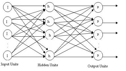Figure 2.2. Back propagation model

The neural network training is conducted based on a back propagation algorithm, with the purpose of adjusting values that are associated to synapses to allow the neural network to map an input space and output space, in which the input vector x are samples of the input space and each input vector is associated to an output z, which can be represented by a vector z (z₁, z₂, ….z_n), based on a scalable value or a symbolic value. During the neural training process, a set of input data is initially determined, too which the association output is known, and random values are attributed to each synapse in the neural network. The data is presented to the neural network and the supplied output is compared to the actual output, generating an error value. The error value is then employed to adjust reverse neural network synapses, from output to inputs (back propagation). Specifically, for symbolic values, a neuron in the output layer corresponds to each of the possible symbols that are associated to the input vector. The process of adjusting synapse value is represented until an interruption criterion is established, for example, a fixed number of repetitions or a minimum error. Thus, in each repetition, the outputs that are provided by the neural network get closer to the actual output. The synapse value correction equations minimize error between the output that is provided by the neural network and actual output.

(4)

Where OUT = the final output of a neuron in the output layer, X = the input vector

W = weight vector ‘w’ between neuron ‘I’ in layer ‘k’ and neuron ‘j’ in layer ‘k+1’

2. Kohonen’s self-organizing mapping: unlike the MLP above reacts in terms of forecast (i.e. which class the company belongs to), the Kohonen’s map response in terms of classification (Perez, 2006). For example, the map will determine a certain number of classes and cluster them to set up some group on it own.

3. perception: is a single – layer neural network with binary output. It iss similar to a ‘back – propagation’ but does not contain hidden layers (Rahimian eta al. 1991). The model utilizes supervised learning and a nonlinear threshold unit: if NET output ≥ Threshold OUT = 1

Otherwise OUT = 0

Mathematical Structure of ANN

Mathematically the model can be written as:

(5)

Where x s the vector of explanatory variable, θ is weight vector (parameter) and is the random error component. Equation is the known function for estimating and predicting from the available data. As such, the model can be formulated as:

(6)

Where:

Y = network output

f = output layer activation function

v_o = output bias

h = hidden layer activation fuction

= hidden unit bias (j = i,…..,m)

n = number of input unit

x_i = input vector

w_ij = weight from input I to hidden unit j

v_j = weight from hidden j to output (j = 1, ….,m)

Learning by gradient descent error minimization

The perception learning rule is an algorithm that adjusts the network weights W_mn to minimize the difference between the actual outputs y_ki and the target t_ki. We can quantify this difference by defining the sum squared error function, summed overall output unit i and all training patterns m:

(7)

It is a general aim of network learning to minimize this error by adjusting the weight w_mn.

Typically we make series of small adjustment to the weight w_mn →w_mn + ∆w_mn until the error E(w_mn) is ‘small enough, we can determine which direction to change the weights in by looking at the gradients (i.e. partial derivations) of E with respect to each weight w_mn.

Then the gradient update equation (with positive learning rate η ) given by

(8)

Optimisee the weights (w) by minimizing ∑(o - η)².

2.3. DA approach Versus ANN as Predictor of Insolvency

Statisticians are being encouraged to apply and test neural networks (Cheng and Titterrington 1994), Warner as Misra (1996). The neural network used in this paper are artificial in that they are algorithm rather than real neural network, DA is one of the most popular techniques used for analyzing insolvency (Perez 2006). The main advantage of the DA approach to predict corporate failure is its ability to reduce a multidimensional problem to a single score with a high level of accuracy. However, DA is subject to a number of restrictive assumptions. First DA requires the decision set which is used for distinguishing between failed and non failed companies be linearly separable. Second, DA does not allow a ration’s signal to vacillate depending on its relationship with another ratio, or set of ratios (Ticehurst & Veal 2000). In practice, a ratio may signal financial distress if it is higher or lower than normal. These problems together with issues such as, bias of extreme data points, the multivariate assumption of normality and equal group variance, may ensure DA is unsuited to the complex nature, boundaries and interrelationships of financial ratios (Coats & Fant 1993). The advantage of Artificial Neural Network is that they do not require the pre-specification of a functional form, or the adoption of restrictive assumptions about the characteristics of statistical distributions of the variables and errors in the model. By their nature, ANN systems are able to work with imprecise variables and with model changes over time. They are also able to adapt to the appearance of new cases which represent changes in the situation (Altman et al, 1993). However, reviews on the accuracy of neural network are mixed. Nag (1991) observed that while the ANN’s prediction error was less than with multiple regression model, the residual autocorrelations of the neural network were higher, indicating that performance may not necessarily be superior. However, Odom & Sharda (1990), Wilson and Sharda (1994), Atman (1993) and Trippi and Turban (1996) all found ANN to be superior to DA.

3. Analysis and Results

A basic step for the analysis of the data is the identification of any significant difference between the two groups of the companies (i.e failed and non-failed). This statistics points out some basic characteristics of each group. In this section, we discuss descriptive statistics, discriminant analysis, neural network results and comparison of all results.

3.1. Discriminant Analysis Output

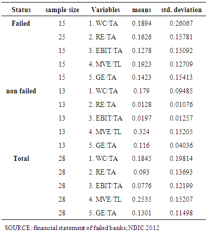
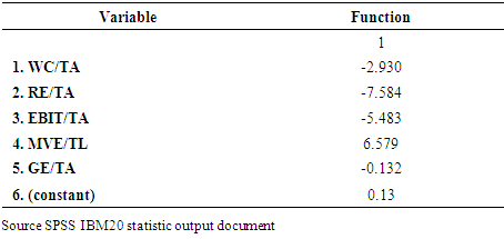
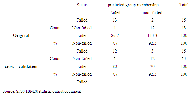
In discriminant analysis, we try to predict a group membership by examining whether there are any significant differences between groups on each of the independent variables using group means data.

Table 1. Summary of Table Bank’s Status

A rough idea of variables that may be important can be obtained by inspecting the group means and standard deviation. Table 1 suggests that these score may be good discriminators as the separations are large.

Group means provide us with a rough idea on how each variable distinguishes between ‘STATUS’. In this case, there is very little difference with regard to group means of ‘WC.TA’ between the two groups, However, we see greater variation between the groups with the variable ‘MVE.TL’.

Table 2. Group Means for Banks’ Status

After examining variability in the ration means, RETA, EBIT/TA, MVE/TL were found to be significant at the 0.05 level, indicating substantial difference in variables between groups. This shows there is significant variety in the ratios of failed and non – failed companies. These finding indicates financial ratios do have significant different predictive abilities for detecting failures of Nigerian finance. Table 3 provides strong statistical evidence of significant difference between means of failed and non-failed groups for all independent variable with RE/TA, EBIT/TA and MVE/TL producing high value F ratio. Large F value indicates that an independent variable has superior discriminatory power.

Table 3. Test of Equity of group means

Having seen the equality of group means, we precede to the inter-correlation, among the independent variables. Table 4 shows that the correlation among independent variable is low; it therefore support the use of the independent variables for the classification of the banks’ status.

Table 4. Correlation between the independent variables

Table 5 provides information on each of the discriminate equation produced. The maximum number of discriminant equation produce is the number of groups minus 1. Only two groups were used here, namely; failed and non – failed, so only one function is displayed. The canonical correlation is the multiple correlations between the predictor and the discriminant function. With only one function it provides an index of overall model fit which is interpreted as being the proportion of variance explained (R²). This report a canonical correlation of 0.805 which suggest that the model explains 64.8% of variation in the grouping variable, i.e whether a financial company failed or not.

Table 5. Eigenvalues

Wilk’s Lambda table indicates the significance of the discriminant function. Table 6 indicates a highly significant function (p<0.05) and provides the proportion of total variability not explained. So we have 35.2% unexplained.

Table 6. Wilks’ Lambda

These unstandardized coefficient b is used to create the discriminant equation, it operates just like a regression equation. In this case, we have;

(9)

The discriminant function coefficients b or standardized from beta both indicate the partial contribution of each variables to the discriminate function controlling for all other variables in the equation. They can be used to access each independent variable’s unique contribution and therefore provide information on the relative importance of each variable. With the DA function, we see that only ‘MVE.TL’ (yielded largest number) may have an important role within our analysis. However, one of the weaknesses of discriminant analysis is the fact that there is no significance test for the coefficients. Thus, we simply look for the highest value as the most important variable. And as this case implies, there is usually some correspondence with the group means results of the test on means.

Table 7. Canonical Disccriminant Function Coefficients

Table 8 below report the prior probability for each group. This number in our case 0.5357 and 0.464 for failed and non-failed banks respectively describe the estimated likelihood that a case belongs to a particular group.

Table 8. Prior Probability for Banks’ status

Here is the classification phase, the classification table also called a confusion table. The percentage cases on the diagonal are the percentages of correct classifications. The cross validation set of data is more honest presentation of the power of the discriminant function than that provided by the original classifications and often produces a poorer outcome The cross validation is often termed a ‘jack- knife’ classification, in that it successively classifies all cases but one to develop a discriminant function and then categorizes the cases that was left out. The classification result in table 9 reveals that 85.7% of banks were classified correctly into ‘failed’ or ‘non – failed’ groups. Non – failed banks are classified with slightly better accuracy (92.3%) failed banks (80%).

3.2. Neural Network Output (One Hidden Layer)

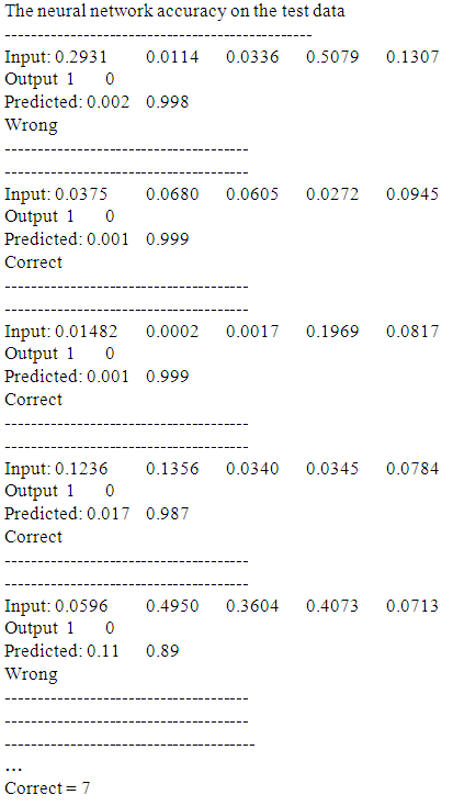
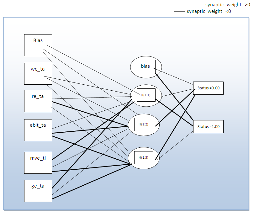
The networks considered in this paper are commonly referred to as multi-layer perception, in that they are organized hierarchically into layers of neurons or nodes.

Goals is to predict output based on 5 inputs

First few rows of raw data file are:

Train and test matrices using a 64.3% 35.7% split

First few rows of training matrix are:

Creating 5 – input 3- hidden 2-output neural network

Best neural network weighs using PSO with cross entropy error final best (smallest) cross entropy error = 0.424

Best weights found:

Table 9. Classification result for Banks’ status

When performing classification analysis with set of existing data, one common approach called holdout validation, is to split the data set into a larger data (18 rows) set for training the neural network and a smaller set (10 rows) for the model. Training means finding the neural weights and bias that minimize some error value. Testing means evaluating the neural network with the best weights found during training. The output above creates a network with five input neurons, three hidden neurons and two output neurons. (5-3-2). The model above correctly predicts 7 of the 10 test vectors. From the test matrix, we have seven correct and three incorrect classification giving rise to 89.3% prediction accuracy of the back propagation network.

Table 10. Input Nodes

The output from summary gives us the detail of the neural network. i₁, i₂, i₃, i₄ and i₅ are the input nodes (WC/TA, RE/TA, EBIT/TA, MVE/TL and GE/TA respectively); O is the output node (STATUS); and b is the bias. Table 4.10 contains weights of the input nodes of WC/TA, RE/TA, EBIT/TA, MVE/TL and GE/TA respectively without the hidden layer while

Table 11. Output Nodes

Table 11 contains the output nodes of WC/TA, RE/TA, EBIT/TA, MVE/TL and GE/TA respectively having the hidden layer (6.02).

The above model -0.06 is bias -0.57, 0.20, 0.14, 0.02 and -0.15 are weights of WC/TA, RE/TA, EBIT/TA, MVE/TL and GE/TA respectively which is synonymous to parameter estimates in statistical terms

MSE

[1] 0.03568584

>AIC2

[1] -84.34233

The mean square error is 0.03569 while the AIC is -84.34233.

Fig. 2.3 consists of a network which is composed of an input layer, which consists of five covariates; WC/TA, RE/TA, EBIT/TA, MVE/TL and GE/TA, a hidden layer with three units; (H (1:1) H (1:2) H (1:3)), a bias and an output layer, with two units 0 and 1. The hidden layers simulate interaction effect amongst the nodes in the layers. In statistical terminology, nodes in the input layer corresponds to the independent variables while nodes in the output layer corresponds to the dependent variable.

Figure 2.3. Output layers activation function

3.3. Comparison of Neural Network and Discriminant Analysis

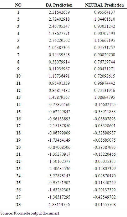
This section compares the testing results derived from failure prediction models developed in this study. Table 12 summarizes the results of these methods. As far as the overall correct classification is concerned, NNs were proved to be superior as the highest prediction results to insolvency.

Table 12. Comparison of both models

The table above shows a summary of the result obtained for DA and neural analysis of the bank data for the prediction of the STATUS of banks in Nigeria. The forecasting ability of the two models is accessed using Mean Absolute Square Error (MSE), and Akaike information criterion (AIC). The results clearly show that neural networks, when trained with sufficient data and proper inputs, can better predict the STATUS. DA techniques is well established, however it forecasting ability is reduced as the data becomes more complex.

Table 13. Prediction table for the two methods

The study is in the process of optimizing the DA model and ‘pruning’ the ANN model (phasing out of neurons that achieve similar performances to provide a simpler model) to achieve greater efficiency of prediction. This indicates that adopting ANN for insolvency prediction is more thorough and a creative process than earlier models and this leads us too accepting our null hypothesis.

4. Conclusions

This study employed financial ratios for differentiating between failed and non-failed financial companies (banks) in Nigeria. These financial variables were derived from the financial statements of failed and non – failed companies. Methodologies adopted include univariate tests, DA and ANN (back propagation algorithm). The univariate test indicates that failed companies’ financial ratios differ significantly from non – failed companies. Failed companies were less profitable and less liquid.

The aim of this study is to adopt a model that will accurately predict failure of financial companies; twenty – eight banks constitute the sample of which fifteen have been indicated as failed and thirteen as non – failed. However, using discriminant analysis. It is observed that the banks can be disaggregated into two distinct classes i.e. those with positive predicting score which rightly fall into category of banks that has not been filed for receivership and those with negative score which fall into category of banks that has been indicated by Central Bank of Nigeria. Following categorization, it can be concluded that the predicting score is a useful toll to identify banks with deteriorating conditions in Nigeria.

Neural network with their flexible non linear modeling capability without the prior knowledge about the nature of the process do provide more accurate estimates, leading to higher classification rates than other traditional statistical methods. Preliminary findings suggest that satisfactory results (85.7%) accuracy of classification) were achieved with a DA model using those five financial ratios which were found earlier to be effective in predicting insolvency in Nigeria, namely: working capital/total assets retained earnings/total assets, EBIT/total assets and market value of equity/total.