Richard Puurbalanta1, Atinuke O. Adebanji2
1University for Development Studies, Faculty of Mathematical Sciences, Department of Statistics, Navrongo Campus, Ghana
2Kwame Nkrumah University of Science and Technology, Faculty of Physical Sciences, College of Science, Department of Mathematics, Kumasi, Ghana
Correspondence to: Richard Puurbalanta, University for Development Studies, Faculty of Mathematical Sciences, Department of Statistics, Navrongo Campus, Ghana.
| Email: |  |
Copyright © 2016 Scientific & Academic Publishing. All Rights Reserved.
This work is licensed under the Creative Commons Attribution International License (CC BY).
http://creativecommons.org/licenses/by/4.0/

Abstract
Though the rate of poverty in Ghana has consistently declined over the years, some parts of the country still record substantially high figures [1], and this is a major concern for stake holders. Previous research to identify causal factors has commonly used the binary logit or probit models. These models, however, mask the effect of important intermediate information during the binary transformation of the response variable. This has the potential to misestimate the probability of poverty. In this study, the ordered probit model was used, thus creating a framework that includes the ordinal nature of poverty severity. The model was based on the round 6 dataset of the Ghana Living Standards Survey. Our findings show that poor and extremely poor were negatively affected by rural location, illiteracy, and Savannah ecological zone. Policies to eradicate poverty must therefore aim at optimizing these significant variables contributions to welfare conditions in the country.
Keywords:
Household Poverty Severity, Predictors, Ordinal Probit Model, MLE, Bayesian estimation
Cite this paper: Richard Puurbalanta, Atinuke O. Adebanji, Household Poverty-Risk Analysis and Prediction Using Bayesian Ordinal Probit Models, International Journal of Statistics and Applications, Vol. 6 No. 6, 2016, pp. 399-407. doi: 10.5923/j.statistics.20160606.09.
1. Introduction
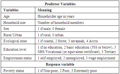
Poverty is the inability to retain a minimal standard of living measured in terms of basic consumption needs or some income required for satisfying them [2]. It is a global development issue [3], and its magnitude and burden is evident, even to the non-observant, especially in developing countries. Thus, the need for research designed to identify the determinants of poverty and to monitor the impact of programs aimed at poverty reduction is imperative.Predictor variables commonly used in poverty studies include socio-economic and demographic attributes of the household [4], which in this study include age, sex, household size, rural/urban location, employment status, and educational level of household head. An additional covariate, ecological zone, was added in this study to estimate the effect of differences in agro-climatic conditions on level of wellbeing. Table 1 gives details of relevant variables extracted from the GLSS dataset for this study.Table 1. Study Variables
 |
| |
|
Previous research to investigate the link between poverty and potential predictors in regression analysis is abundant in the literatures, albeit with varying degrees of sophistication and often with mixed conclusions. For instance, [5] used the logistic regression model to identify household-level determinants of poverty in Albania, and concluded that the probability of being poor is influenced mainly by education and employment status of household head, the household composition and geographic divisions. Dudek and Lisicka [6] used the binary logit model but included interaction terms to describe poverty in Poland. They found that the probability of being poor is influenced by size of the household, living in a rural area, and working in manual positions. Akin to these findings, a recent study in Ghana by [7] using logistic regression to estimate the probability of being in poverty based on living standards survey (LSS) data, reported that large households, and households headed by illiterates negatively affect poverty levels in the country. An important and a notable conclusion reached in their study identified households in the savannah ecological zone of Ghana to be almost four times poorer than those living in the coastal and forest zones. Most studies, including this one, have used household income or expenditure to measure poverty. A common approach has been to dichotomize the dependent variable into poor or non-poor, and use the binary logit or probit models (being the natural choices) to estimate the probability of a household being in poverty. These binary models, however, usually mask the effect of important intermediate information during the binary transformation of the response variable. This has the potential for incomplete and inaccurate conclusions. What we do differently in this study is to adopt a framework for poverty analysis that allows for the response variable to assume all of its key response categories; “non-poor”, “poor”, and “extremely poor” [1]. We then use the proportional odds ordered probit (OP) model [8], thus creating a framework that includes the ordinal nature of poverty severity. This approach allows thorough investigations to determine whether or not distances between the poverty categories differ, and the probability of slipping into the next category given that an individual is already in a lower-risk category, and vice versa. The few previous studies that have used multi-classification methods to model poverty have largely ignored the ordinal nature of the variable. For example, in separate studies, [9] and [10] used a multinomial econometric approach in their bit to quantify the relationship between poverty and socio-economic and demographic variables. The intention to include the multi-categorical nature of poverty was explicit. However, the natural ordering of the variable was ignored. This can easily bias results of the study. The ordered probit (OP) model is an extension of the ordinary binary probit model. It is generally used when categories of the dependent variable exceeds two, and follow a natural order. Ordered models are generally derived within a framework of unobservable underlying latent processes generating observable ordered outcomes. Although it is generally not possible to observe the latent variable, we make the assumption that some factors jointly determine its behaviour. Thus, the latent variable is assumed to be a random function. In this setting, the goal is to understand the influence of the latency on the probability of observing a particular outcome based on individual-related factors.Proportional odds ordered probit models describe the relationship between covariates and the probability to be in a higher ordered category [1]. Intercepts for each comparison is different, but share the same set of estimated beta coefficients. The intercepts show the effect when X = 0. Unlike the partial proportional odds (PPO) model [11] and the generalized ordered probit (GOP) model [12], proportional odds ordered probit models are less complicated and simple to interpret. Estimation of categorical ordered models can be challenging because non-linear optimization methods are involved in the process. Moreover, the regression-based ordered probit model has a unique feature that includes the thresholds as part of unknown parameters to be estimated. This further complicates the estimation process: because of possible unequal spacing between categories, ordinary least squares (OLS) regression, which, theoretically, requires equal interval widths to function properly, is inappropriate. However,  OLS regression becomes legitimate. Additionally, thorough procedures to fest predictability of the model is absent in OLS regression. This is important because the primary aim is to use the developed models for prediction of the unobserved. For these reasons, we employ the Bayesian paradigm for parameter estimation and inference instead of the traditional ordinary least squares (OLS) approach. Bayesian estimation in particular is attractive largely because the latent variable is naturally incorporated as an additional parameter via data augmentation. With advancement in computing power, and the advent of Markov Chain Monte Carlo (MCMC) [13], implementation of the Bayesian framework is easy. A key advantage of Bayesian inference is to fully account for parameter uncertainty associated with the predicted values [14]. Besides, Bayesian inference is robust, and does not need to satisfy any regularity conditions to function properly. The primary objective is to attempt to provide a full description of the character of poverty in a simple and straightforward language, and predict the probability of an unobserved household being in a particular severity category given some covariate characteristics of households in the study area. This way, even non-technical end-users such as government and social-support groups can understand how patterns of economic, social and demographic changes affect different classes of the poor in the country, helping to avoid blanket approach to combating poverty. We base our inference on the latest Ghana living standards survey (GLSS) dataset collected in 2012.
2. Measurement of Poverty
This work, in line with the Ghana Statistical Service (GSS), and following international common practice, adopts monetary measures of poverty. This approach measures poverty in relation to the amount of money necessary to meet some basic consumption needs such as food, clothing, and shelter [15]. Estimation of monetary measures of poverty requires us to choose between disposable income and total consumption expenditure as the indicator of wealth, the latter being the preferred choice in most developing countries, and in this study [1].Moreover, to measure monetary poverty, we need to set minimum standards of the poverty indicator to separate the various categories of the poor from the non-poor. These are called poverty lines [15, 1]. The three categories of poverty lines proposed by [15] are based on family daily expenditure per adult equivalent. Households who spend at least $1.25 a day are non-poor, whiles those who spend less than $1.25 are poor. The extremely poor are those with expenditure less than $1 a day. In Ghana, these thresholds are set at GHC 3.60 per day- non-poor, less than GHC3.60 –poor, and GHC2.17- extremely poor [1].
3. The Ordinal Probit Model
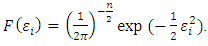
The ordinal probit (OP) model derives from the multinomial distribution, albeit with ranked categories, thus, its likelihood function is multinomially distributed. The multinomial distribution is an extension of the binomial distribution where, now, the number of parameters being modelled exceeds one. The density function for the multinomial distribution is: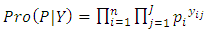 | (1) |
To derive the cumulative ordinal probit (OP) generalized linear model (GLM) from the multinomial distribution, let the responses  be arranged in order of magnitude, and
  the corresponding thresholds associated with the ordering. Further let
  be a Gaussian random variable assumed to be latent [8, 16], and assigning values to
  according to a regression function:
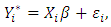 | (2) |
where  is
is  design matrix,
  is a
is a  unknown vector of regression coefficients, and
  is the
  vector of independently and identically distributed
  measurement errors:
  Though the values of
  cannot be directly observed, the rule that assigns
  to
to  is that if
  exceeds a given threshold, then, for example, a household falls in the
  category of poverty. This culminates in cumulative multiple binary outcomes:
 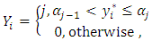 | (3) |
where  and
and 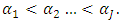 Cleary,
  in our application, refers to the Gaussian expenditure line, and is asymptotic of the ordinal variable
  when
when  Our objective is to predict the probability of a household falling in or below the
  category given the observed covariates
  This probability is determined by the values of the latent variable
  and is given by
 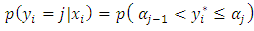 | (4) |
Since  is Gaussian, and
  is assumed to be normally distributed, the outcome is a probit model, implying that the probability of falling in or below the
  category is:
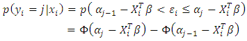 | (5) |
where  is the cumulative distribution function
  for the standard normal
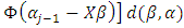
 Thus, the likelihood function for the parameters is
  | (6) |
3.1. Distributional Assumptions and Normalizations of the OP Model
Several normalizations are often needed to identify the ordered model parameters. First, to preserve the positive signs of all the probabilities, it is required that  Second, if the support for the categories is to be the entire real line, then
  and
and  Third, following standard practice, we assume the continuous latent variable
  is standard normal [8, 16].Finally, we assume, following [8], and [16], that
  contains a constant term. Then it is required for
  If this restriction is not imposed, adding a constant to
  and another constant to the vector of beta coefficients results in identifiability problems (the model may appear to contain two constant terms or intercepts).
3.2. Parameter Estimation and Inference
3.2.1. Maximum Likelihood Estimation (MLE)
In our poverty severity application, given that our response is multinomial ordered with  observations and
  categories, where
  and
and  we use the likelihood function for the OP model derived from (1):
  | (7) |
the log-likelihood being 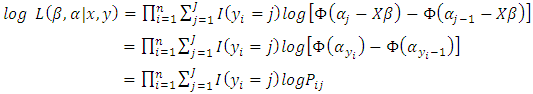 | (8) |
where  is the identity matrix. The ML process chooses that estimators,
  and
and  of the set of unknown parameters,
  which maximize the data [17, 18, 16]. Like many models, the curve of
  is non-linear [16] and
  and
and  is the point at which
 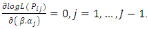 | (9) |
Equation (9) is maximized to obtain the MLE of  subject to
 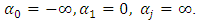 This equation cannot easily be solved analytically. So we adopt the Newton-Raphson iterative algorithm [8]. A measure of how well the model fits is important, and is determined by the significance of the overall model fit statistic. Fit indices include the likelihood ratio test, which is approximately chi-square
 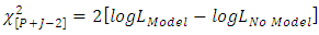 for large
3.2.2. Bayesian Estimation via Gibbs Sampling
Following the Bayesian criteria, we set priors for the parameters, and build the posterior as: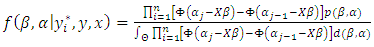 | (10) |
where 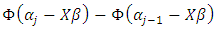 is the data likelihood,
  is the density of the prior, and
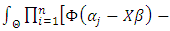
 is the integrated likelihood with
  being the parameter space.The
  matrix of beta coefficients
  arises from the mean structure of the multivariate latent multivariate Gaussian variable
  , so we assign a multivariate prior
  where
where  is the mean and
  is the covariance matrix. If
  is small
  is large, this becomes non-informative prior.The thresholds
  where
where  and
and  for
for  are jointly distributed with
  We therefor impose a conjugate multivariate normal distribution on
  where
where  vector and
  is diagonal matrix. For
  and
and  this is also a non-informative prior.The unknown values
  are treated as nuisance parameters to be estimated along with
  Conditional on
  and
and  is a truncated normally distributed variable with mean
  and variance 1. That is, the latent variable has a multivariate normal prior distribution with density:
  | (11) |
where  is the mean, and
  is the variance. This is a doubly truncated normal distribution (truncated to the left by
  and to the right by
  ). Posterior estimation is done by setting up the Gibbs sampler [19], which requires us to derive full conditionals for all parameters:
  | (12) |
 | (13) |
where  is an indicator variable. The likelihood function of
  is thus
 | (14) |
where  vector of ones,
  and
and  for
for  Thus, we obtain the full conditional posterior of
  conditioned on
 | (15) |
This is a truncated normal distribution. We allow  whiles
  to impose vague prior on
  Thus,
Thus, | (16) |
MCMC techniques then make draws from the uniform distribution in the interval:
 | (17) |
The Gibbs algorithm to generate posterior samples is extended in the following steps:i. Choose initial values for all parameters including thresholds. ii. Sample the latent variable  from truncated normal distributions on the truncation interval
  iii. Sample thresholds
  from uniform distributions on the interval
  iv. Sample the regression coefficients from
  v. Repeat the steps until enough samples are drawn for inference.
3.3. Posterior Predictions and Model Evaluation
Predictions of the unobserved  are made using the posterior predictive density:
 | (18) |
where  is the parameter space. The posterior predictive density is the distribution of possible future observations that could arise from the current model.Subsequently, it is important to assess whether the model built fits the data sufficiently for prediction within and, possibly, beyond the observed data. That is, we determine a checking function for both predicted data and actual observations to assess whether the predictive model adequately reproduces at least some key features of the actual observations to conclude the model fits well. In standard ML analyses, a repertoire of fit measures includes
  and likelihood-ratio
  statistics. In Bayesian analyses, predictive model selection is checked within the framework of Bayesian decision theory [20], where prediction accuracy is based on the Bayesian expected loss (the expected value of the loss function given the data) [20]. The loss function
  represented here by the squared prediction error loss, assigns zero loss to correct predictions [21]. For the multi-categorical application, the Bayesian expected loss is expressed as
  | (19) |
The optimal Bayes predictor (the category with the largest probability) is found at  where
where  is at its minimum. Alternative procedures to measure fit include Bayesian p-values. To calculate the p-value, we first define a test statistic
  (high values of which show poor fit) to be a function of the data, and
  to be the same function but applied to simulated or training data. We then compute the Bayesian p-value as:
 | (20) |
Equation (20) represents the proportion of simulated future datasets whose functional values  exceed that of the function
  applied to the original data. That is, the probability that a future observation would exceed the observed data, given the model. So, an extreme p-value implies poor model fit [22]. We jointly apply the two fit measures (Bayesian expected loss and Bayesian p-value) to determine the model’s ability to forecast future values.
4. Data Description
The study used secondary data from the Ghana Living Standard round 6 Survey. The Ghana Living Standard Survey (GLSS) focuses on the household as the socioeconomic unit, but collects information on individuals within the household and on the communities in which the households are identified. Data are gathered on wide ranging issues including demographic characteristics, education, economic activities, and health. For the GLSS round 6, a total of 16772 households were sampled across Ghana. Cumulative proportional odds probit models are constructed to categorize households using a set of cut-point values (non-poor, poor, and extremely poor) based on the micro data of the GLSS.
5. Preliminary Analysis
In this section, we examine the relationship between poverty and its correlates using the ordered probit model. We subject the model to relevant cross-validation tests by randomly splitting our dataset into two parts: one part (5000) as hold-out set and the other (11772) as validation set. Our sample size of 16772 is relatively large to permit a hold-out dataset. We use comparisons of the two datasets to investigate the model’s ability to estimate parameters and accurately predict future observations under similar conditions. This step is important [23], especially when dealing with non-Gaussian models. First, using the hold-out set, we conducted a graphical analysis to test conformity of the model with the proportional odds assumptions [17]; the assumption that independent variables’ effect on the cumulative odds does not change from one cumulative odds to the next. Results obtained show a fairly affirmative picture (Figure 1). Some deviations were observed in the effects of location and ecological zone, though.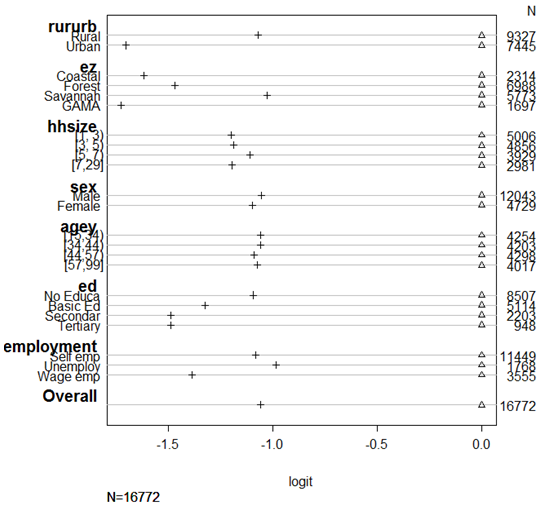 | Figure 1. Test of Proportional Odds Assumption |
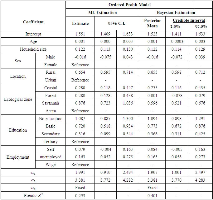
Next, to examine the usefulness of the model for prediction, we fit a one-covariate model to the hold-out dataset. The model was fit using the procedure detailed in this study and implemented in [24]. We ran the MCMC chain for 10000 iterations. Posterior summaries for prediction and estimation were based on the last 5000 iterations of the chain.Summaries of results for Bayesian expected loss (BEL) (0.21), and Bayesian p-value (0.364) show that the model appears very effective in predicting unobserved values, the low BEL values indicating barely noticeable mis-prediction losses.Using 95% posterior credible intervals to summarize the range of possible values (Table 2), it is obvious that the model was successful at capturing the data-generating process. This means that the model provides correct conclusions about the association between the response and the predictor.Table 2. ML and MCMC Estimates for the Ordinal Probit Model
 |
| |
|
6. Model Results
In this section, we fit the model on the remaining dataset. Inference compared MCMC simulations (via Gibbs sampling) with the commonly used ML estimation. Results of the two models were generally identical. However, the Bayesian  value of 0.401 shows that the Bayesian model is superior to the ML model
  More importantly, the Bayesian expected loss
  and p-value
  show that the Bayesian model is suitable for parameter estimation and prediction. For the MLE, coefficients of the threshold are
  and
and  and differ significantly from each other (Table 2), with
  (poor) being more likely regardless of the covariates. The threshold values for the Bayesian model are similarly distributed (Table 2), so the use of the ordered probit model that categorizes the poor according to severity levels is better than using a single model to describe poverty. The observed differences in the threshold parameters basically reflect the differential parameterizations between the two approaches.Table 2 summarizes and compares results of ML estimates and the Bayesian inference. The results show that all but the coefficients for sex, age and self-employment were statistically significant in both models. Whiles forest ecological zone was statistically significant in the ML model, its contribution to the Bayesian model was negligible. Many of the statistically significant covariates were generally strongly related with the response variable. The coefficient of the variable household size for example, is statistically significant in both models; its contribution to change in log-odds ratio being 1.130. The impact of a unit change in the variable no education on the log-odds of a change in economic status is similarly high (OR = 2.965 for the MLE and OR = 2.986 for the Bayesian model). The converse is true for households whose heads have higher education. Using Tertiary education as reference, and the ML model, the odds ratios are 2.965, 2.054, and 1.372 for no education, basic, and secondary education. Living in the savannah ecological zone or rural place negatively impacts the log-odds of poverty among households in Ghana by 2.401 and 1.923 respectively. We also observed strong association between poverty severity and location (Rural/Urban). The estimated model is given in Table 2. Marginal effects of the covariates were estimated for the Bayesian model (Table 3). In ordered modelling, a unit increase in the independent variable changes the probability of falling in the
  alternative by the marginal effect in percentage terms. For this study, results of Table 3 show that every one unit increase in household size decreases the probability of falling in the non-poor category by 2.8%, but increases the probability of poor and extremely poor by 1.9% and 0.09% respectively, implying that a 1 unit increase in household size tends to deteriorate the economic conditions of households (from non-poor through poor to extremely poor).
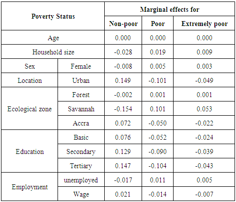
Table 3. Marginal Effects for the Bayesian Ordinal Probit Model
 |
| |
|
Moreover, urban location increases the probability of non-poor by 14.9%, but is associated with being 10.1% and 4.9% more likely to be in the poor or extremely poor categories respectively. Similarly, having a higher level of education significantly decreases the expected levels of poverty on the log-odds scale, tertiary education contributing the largest in this respect.Based on results of Table 2, the Bayesian ordered probit (BOP) model equations for prediction are: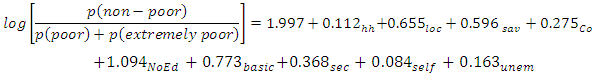 | (21) |
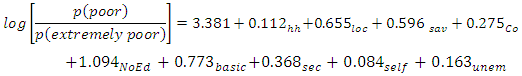 | (22) |
where  Household size,
  location (rural/urban),
  savannah ecological zone,
  coastal ecological zone,
  No education,
  Basic level education,
  Secondary school certificate, and
  self-employed,
  unemployed.Predictions using (17) show that for a Ghanaian, the probability of being non-poor, poor or extremely poor, respectively, are 75.93%, 14.15% and 9.92%.Figure 2 presents results to compare predicted and expected probabilities of falling into poverty.
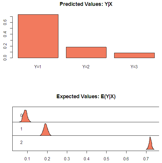 | Figure 2. Predicted and Expected Probabilities of Falling in a Poverty Category |
7. Discussion
The study employed the proportional odds cumulative probit model that ordered the population into three distinct categories (non-poor, poor, and extremely poor). The model was built to forecast the risk of household poverty in Ghana. Inference compared MCMC simulations (via Gibbs sampling) with the commonly used ML estimation. A key difference between the Gibbs sampler and that for the ML is the necessity to sample latent data from doubly truncated normal distributions. Though results were generally identical, the Bayesian  value of 0.401 shows that the Bayesian model is superior to the ML model with a
  value of 0.310. The estimated marginal effects clearly highlighted the strong association between poverty and its correlates. Similar findings were made by [25] who used both a bivariate and an ordered probit model to estimate the effects of different socio-economic and demographic variables on the probability of a household being in poverty in Malaysia. In their analyses, the authors found that the probability of being in poverty was higher for rural families. [26] also applied the binary logit model to assess the causal relationship between poverty and some household-specific economic and demographic explanatory variables in Nigeria. They similarly found that being located in a rural community and having a large household size significantly increases the probability of falling below the poverty line. Many other studies have shown poverty to be predominantly rural and affected by large household size [5, 6]. Furthermore, our estimation results show significant variations in the relationship of the response variable with the different levels of categorical covariates. We see in Table 2, for example, that effect of the coefficients for education are inversely related to the probability of poverty, reducing the likelihood of dropping from non-poor to poor or extremely poor as education advances. This scenario was also found with the ecological zone variable. The high log-odds ratio value of the savannah ecological zone variable corroborate the work of [7] who reported that households in the savannah ecological zone of Ghana were almost four times poorer than those living in the coastal and forest zones in 2005/06. This could be attributed to the fact that the seaports and heavy industrial plants (along with the recently discovered crude oil) are found predominantly across the middle and coastal belts of the country, where both the rich agricultural lands and tropical rain forest coincide. We also observe that being male reduced the risk of falling into poor or extremely poor 0.984. This finding is consistent with the work of [26] in Nigeria, who concluded that households with female heads were more likely to be poorer. This variable’s effect is, however, not statistically significant.
8. Conclusions
The results we obtained show that out of the seven observed covariates, age, sex, as well as one level of ecological zone (forest) and self-employed do not significantly affect the distribution of household poverty in Ghana. The most powerful predictors of extreme poverty include rural location, Savannah ecological zone and household heads with little or no education. We therefore entreat pro-education and pro-rural development agencies such as the Savannah Accelerated Development Authority (SADA) to intensify efforts aimed at combating poverty. We also recommend more diverse research into the area because the ability to correctly predict who is at risk should be the first step, and an integral part of efforts to combat poverty.To improve parameter estimation, since the data was collected at different geographical locations, further research into the area using spatial analysis tools, instead of the standard regression methods used in this study, is recommended.
References
| [1] | Ghana Statistical Service (2014). Poverty Profile in Ghana. http://www.statsghana.gov.gh/docfiles/glss6/GLSS6_Poverty%20Profile%20in%20Ghana.pdf. |
| [2] | Townsend, P. (2014). International Analysis Poverty. Routledge. |
| [3] | United Nations Development Programme (2010). What Will It Take to Achieve the Millennium Development Goals?– An International Assessment. |
| [4] | United Nations Development Programme (2014). Summary: Human Development Report 2014; Sustaining Human Progress: Reducing Vulnerabilities and Building Resilience |
| [5] | Tomori, M., Elena, Zyka, E., & Bici, R. (2014). Identifying Household Level Determinants of Poverty in Albania Using Logistic Regression Model (SSRN Scholarly Paper No. ID 2457441). Rochester, NY: Social Science Research Network. |
| [6] | Dudek, H., & Lisicka, I. (2013). Determinants of poverty–binary logit model with interaction terms approach. Ekonometria, (3 (41), 65–77. |
| [7] | Ennin C.C., Nyarko P.K., Agyeman A., Mettle F.O., Nortey E.N.N. (2011). Trend Analysis of Determinants of Poverty in Ghana: Logit Approach. Research Journal of Mathematics and Statistics 3(1): 20-27, 2011, ISSN: 2040-7505. |
| [8] | Agresti, A. (2007). An Introduction to Categorical Data Analysis. Wiley. |
| [9] | Umer Khalid, Lubna Shahnaz and Hajira Bibi (2005). Determinants of Poverty in Pakistan: A Multinomial Logit Approach. The Lahore Journal of Economics. 10 : 1 (Summer 2005) pp. 65-81 |
| [10] | Samir B-E. Maliki, Abderrezak Benhabib, Abdelnacer Boutedja (2012). Quantification of the Relationship Poverty Education in Algeria: A Multinomial Econometric Approach. Topics in Middle Eastern and North African Economies, electronic journal, Volume 14, Middle East Economic Association and Loyola University Chicago, September, 2012, http://www.luc.edu/orgs/meea/. |
| [11] | Fullerton A. S., 2009. A conceptual framework for ordered logistic regression models. Sociological methods and research 38 (2), 306-47. |
| [12] | Terza, J. V., 1985. Ordinal probit: a generalization. Communications in Statistics-Theory and Methods 14 (1), 1-11. |
| [13] | Gelfand, A.E. and A.F.M. Smith. (1990). “Sampling-Based Approaches to Calculating Marginal Densities.” Journal of the American Statistical Association. |
| [14] | Garthwaite, P., Kadane, J. and O’Hagan, A. (2004) Elicitation Journal of the American Statistical Association. |
| [15] | Ravallion, Martin; Chen, Shaohua; Sangraula, Prem (May 2008). Dollar a Day Revisited (Report). Washington DC: The World Bank. |
| [16] | William H. Greene, David A. Hensher (2009). Modeling Ordered Choices. |
| [17] | McCullagh, P., 1980. Regression models for ordinal data. Journal of the Royal Statistical Society, 42 (2), 109-142. |
| [18] | Lance A. Waller, Carol A. Gotway (2004): Applied Spatial Statistics for Public Health Data. John Wiley & Sons, Inc., Hoboken, New Jersey. Pp 327. |
| [19] | Stuart Geman and Donald Geman, (1984). Stochastic relaxation, Gibbs distributions, and the Bayesian restoration of images. IEEE. |
| [20] | Geisser, S. and Eddy, W. (1979) A predictive approach to model selection. |
| [21] | Berger, J.., 1985. Statistical Decision Theory and Bayesian Analysis. Springer Verlag, New York, New York, USA. |
| [22] | Rubin, D.B. 1984. “Bayesianly Justifiable and Relevant Frequency Calculations for the Applied Statistician.” Annals of Statistics 12:1151–1172. |
| [23] | Lewis, S. and Raftery, A. (1997) Estimating Bayes factors via posterior simulation with the Laplace-Metropolis estimator. Journal of the American Statistical Association, 92, 648–655. |
| [24] | R Development Core Team, 2007. R: A Language and Environment for Statistical Computing. R Foundation for Statistical Computing, Vienna, Austria, ISBN 3-900051-07-0. URL http://www.R-project.org. |
| [25] | Saidatulakmal and Madiha Riaz (2012). Demographic Analysis of Poverty, Rural-Urban Nexus. Research on Humanities and Social Sciences. Vol.2, No.6, 2012. |
| [26] | Osowole, O.I., Ugbechie, Rita, Uba, Ezenwanyi (2012). On The Identification of Core Determinants of Poverty: A Logistic Regression Approach. Mathematical Theory and Modeling. Vol.2, No.10, 2012. |

 Abstract
 Reference
 Full-Text PDF
 Full-text HTML