Najrullah Khan, Md. Tanwir Akhtar, Athar Ali Khan
Department of Statistics and Operations Research, Aligarh Muslim University, Aligarh, India
Correspondence to: Najrullah Khan, Department of Statistics and Operations Research, Aligarh Muslim University, Aligarh, India.
| Email: |  |
Copyright © 2016 Scientific & Academic Publishing. All Rights Reserved.
This work is licensed under the Creative Commons Attribution International License (CC BY).
http://creativecommons.org/licenses/by/4.0/

Abstract
The Inverse Gaussian distribution is a plausible model in settings where failure occurs when a deterioration process reaches a certain level. More generally, it is a reasonably flexible two-parameters family of models with properties that are rather similar to those of log-normal distribution. In this paper, an attempt has been made to outline how the Bayesian approach proceeds to fit such a model using Laplace Approximation, which requires the ability to maximize the joint log-posterior density. This model is applied to a real survival censored data, so that, all the concepts and computations will be around that data. R code has been developed and provided to implement in censored mechanism using analytic Laplace Approximation method. Moreover, parallel simulations tools are also implemented with an extensive use of R.
Keywords:
Inverse Gaussian Model, Laplace Approximation, Posterior, Simulation, LaplacesDemon, R
Cite this paper: Najrullah Khan, Md. Tanwir Akhtar, Athar Ali Khan, A Bayesian Approach to Survival Analysis of Inverse Gaussian Model with Laplace Approximation, International Journal of Statistics and Applications, Vol. 6 No. 6, 2016, pp. 391-398. doi: 10.5923/j.statistics.20160606.08.
1. Introduction
Survival analysis is a collection of statistical procedures for data analysis for which the outcome variable of interest is time until an event occurs, for example, death of a patient, time to first recurrence of a tumor after initial treatment, time to the learning of a skill and promotion time for employees. Survival analysis arises in many fields of study including medicine, biology, engineering, public health, epidemiology and economics. Various models exist that are commonly used in survival analysis, for example, Weibull, normal and gamma distributions. Another important model for survival data is inverse Gaussian distribution. The Inverse Gaussian distribution is a plausible and reasonably flexible two-parameters family of models with properties that are rather similar to those of log-normal distribution. In this paper, an attempt has been made to outline how Bayesian approach proceeds to fit Inverse Gaussian model for lifetime data using LaplaceApproximation, which required the ability to maximize the joint log posterior densities. The tools and techniques used in this paper are in Bayesian environment, which are implemented using LaplacesDemon package of Statisticat (Statisticat LLC 2014). Goal of this package is to provide a complete and self-contained Bayesian environment within R and approximate the posterior densities using one of the Markov chain Monte Carlo(MCMC) algorithms.The function LaplaceApproximation of LaplacesDemon approximates the posterior results analytically and then after convergence it gives simulated results using sampling importance resampling (SIR) method. In LaplaceApproximation function there is an argument called "Method". The method used to approximate posterior density is the Trust Region(TR) algorithm of Nocedal and Wright (1999) is used. The TR algorithm attempts to reach its objective in the fewest number of iterations, is therefore very efficient, as well as safe. The efficiency of TR is attractive when model evaluations are expensive. Another main function of this package is LaplacesDemon, which maximizes the logarithm of unnormalized joint posterior density using one of the MCMC algorithms. In LaplacesDemon the algorithm used for simulation is Independent Metropolis. This package does not deal with censoring mechanism. We have developed function for censored data which works well for the analysis of survival data. Real survival data is used for the purpose of illustration. Thus, Bayesian analysis of inverse Gaussian distribution has been made with the following objectives:• To define a Bayesian model, that is, specification of likelihood and prior distribution.• To write down the R code for approximating posterior densities with Laplace Approximation and simulation tools.• To illustrate numeric as well as graphic summaries of the posterior densities.
2. The Inverse Gaussian Distribution
The Inverse Gaussian distribution is a plausible model in settings where failure occurs when a deterioration process reaches a certain level. More generally, it is a reasonably flexible two-parameters family of models with properties that are rather similar to those of log-normal distribution. If T has Inverse Gaussian Distribution, we denote this by (Meeker and Escobar, 1998). The InvG cdf, pdf and survival function are respectively:
  Where
Where  As
As  tends to infinity, the inverse Gaussian distribution becomes more likely to a normal distribution as it is evident from Figure 1.
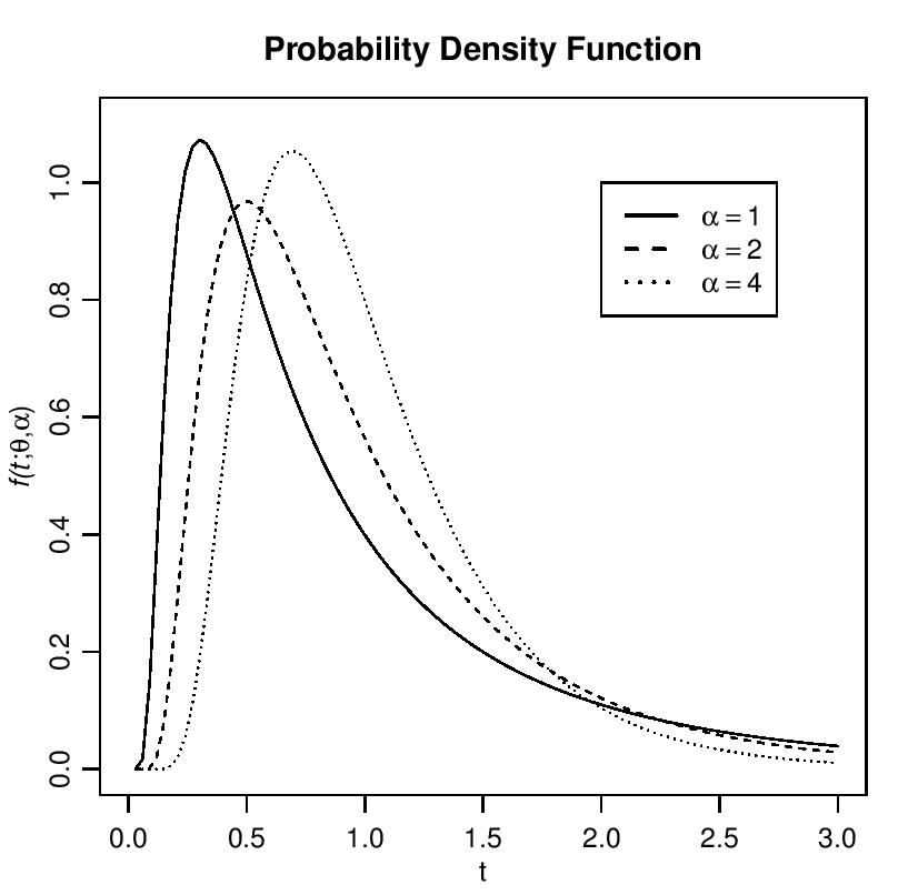 | Figure 1. Probability density function of inverse Gaussian Distribution for α = 1, 2, 4 |
3. The Prior Distributions
In Bayesian paradigm, it is needed to specify prior information regarding the value of the parameter of interest or information that is available before analyzing the experimental data by using a probability distribution function. This probability distribution function is called the prior probability distribution, or simply the prior, since it reflects information about parameter prior to observing experimental data. Here some prior distributions are discussed according to their uses in subsequent Bayesian reliability models.
3.1. Weakly Informative Priors
Weakly Informative Prior (WIP) distribution uses prior information for regularization and stabilization, providing enough prior information to prevent results that contradict our knowledge or problems such as an algorithmic failure to explore the state-space. Another goal is for WIPs to use less prior information than is actually available. A WIP should provide some of the benefit of prior information while avoiding some of the risk from using information that doesn’t exist (Statisticat LLC, 2013). A popular WIP for a centered and scaled predictor (Gelman, 2008) may be θ ∼ N(0,10000)), where θ is normally-distributed according to a mean of 0 and a variance of 10,000, which is equivalent to a standard deviation of 100 or precision of 1.0 10-4. In this case, the density for θ is nearly flat. Prior distributions that are not completely flat provide enough information for the numerical approximation algorithm to continue to explore the target density, the posterior distribution.
3.2. The Half-Cauchy Prior Distribution
The probability density function of half-Cauchy distribution with scale parameter α is given by 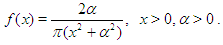 The mean and variance of the half-Cauchy distribution do not exist, but its mode is equal to 0. The half-Cauchy distribution with scale α = 25 is a recommended, default, noninformative prior distribution for a scale parameter. At this scale α = 25, the density of half-Cauchy is nearly flat but not completely (see Figure 2), prior distributions that are not completely flat provide enough information for the numerical approximation algorithm to continue to explore the target density, the posterior distribution. The inverse-gamma is often used as a noninformative prior distribution for scale parameter, however, this model creates problem for scale parameters near zero, Gelman and Hill (2007) recommend that, the uniform, or if more information is necessary the half-Cauchy is a better choice. Thus, in this paper, the half-Cauchy distribution with scale parameter α = 25 is used as a noninformative prior distribution (Akhtar and Khan, 2014 a, b).
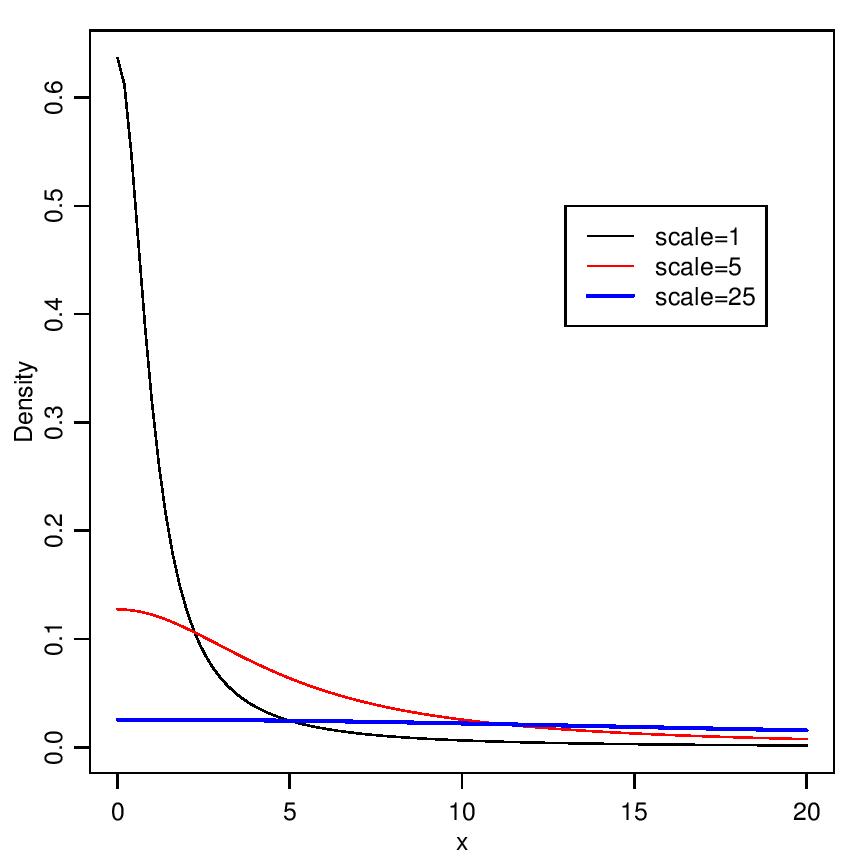 | Figure 2. It is evident from the above plot that for scale=25 the half-Cauchy distribution becomes almost uniform |
4. The Laplace Approximation
Many simple Bayesian analyses based on noninformative prior distribution give similar results to standard non-Bayesian approaches, for example, the posterior t-interval for the normal mean with unknown variance. The extent to which a noninformative prior distribution can be justified as an objective assumption depends on the amount of information available in the data; in the simple cases as the sample size n increases, the influence of the prior distribution on posterior inference decreases. These ideas, sometime referred to as asymptotic approximation theory because they refer to properties that hold in the limit as n becomes large. Thus, a remarkable method of asymptotic approximation is the Laplace Approximation which accurately approximates the unimodal posterior moments and marginal posterior densities in many cases. In this section we introduce a brief, informal description of Laplace approximation method.Suppose -h(θ) is a smooth, bounded unimodal function, with a maximum at  and θ is a scalar. By Laplace’s method (e.g., Tierney and Kadane, 1986), the integral
 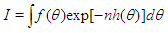 can be approximated by
  where,
 As presented in Mosteller and Wallace (1964), Laplace’s method is to expand about
  to obtain:
 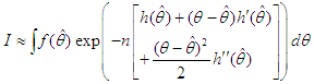 Recalling that
  we have
 Intuitively, if
  is very peaked about
  then the integral can be well approximated by the behavior of the integrand near
  More formally, it can be shown that
 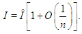 To calculate moments of posterior distributions, we need to evaluate expressions such as:
 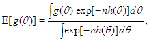 | (1) |
where  (e.g., Tanner, 1996).
5. Bayesian Analysis of Inverse Gaussian Model
5.1. The Model
Over a century the family of Inverse Gaussian distribution has attracted the attention of many researchers in several fields specially in reliability as well as survival analysis because of its  -shape of hazard rate function like log-normal, generalized Weibull and log-logistic distribution. That is, the hazard rate of inverse Gaussian distribution is unimodal which increases from 0 to its maximum and then decreases asymptotically to a fixed value (constant). In other worlds, the inverse Gaussian distribution has one mode in the interior of the values of possible values and it is skewed to the right, sometimes with an extremely large tail. The fact that extremely large outcome can occur when almost all outcomes are small is a distinguish characteristic.It is more convenient to define the model in terms of the parameterizations
  leading to
 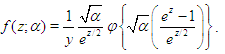 | (2) |
Throughout we use the notation  , where
  to denote the density (Equation 2). Let
 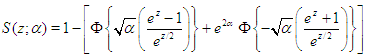 | (3) |
denote the survival function. We can write the likelihood function of  for right censored (as is our case the data are right censored) as
 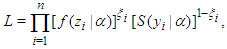 | (4) |
where  is an indicator variable which takes value 0 observation is censored and 1 otherwise. Thus, the likelihood is given by
 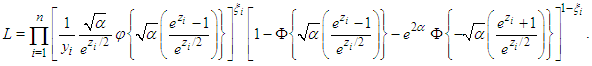 where
where 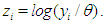 Subsequently, to built the inverse Gaussian regression model, we introduce covariate through
  with function and write
  Moreover, to compare the model in Bayesian paradigm, it is important to choose an appropriate prior distributions for regression coefficients
  and shape parameter
  , according to available information. Making the choice is a challenge because
  parameters have support on real line and
  on positive real line. For this situation, separate and independent priors should be chosen. One choice on prior for
  parameter is
  which is normal distribution with mean 0 and large variance 1000 or a small precision 1 10-3. The density for
  with large variance is nearly flat. Priors that are not completely flat provide enough information for the numerical approximation to contribute to explore the target density. Similarly, for the shape parameter
  the choice of prior is half-Cauchy with scale
  that is,
  Thus, using these prior distributions the joint posterior density is
  which is not in closed form. Consequently, the marginal posterior densities of parameters
  and
and  are also not in closed form. These marginal densities are the basis of Bayesian inference and therefore one needs to use numerical integration or MCMC methods. Due to the availability of computational tool like R and LaplacesDemon, the required model can easily be fitted in Bayesian paradigm using LaplaceApproximation as well as MCMC techniques.
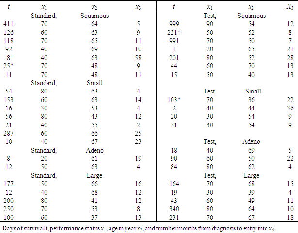
5.2. The Data: Lung Cancer Survival Data
Let us introduce a lifetime dataset taken from Lawless (1982), so that all the concepts and computations will be discussed around that data. Lung cancer survival data for patients assigned to one of two chemotherapy treatments. The data, given in Table 1, include observations on 40 patients: 21 were given one treatment (standard), and 19 the other (test). Several factors thought to be relevant to an individual’s prognosis were also recorded for each patient. These include performance status  at diagnosis (a measure of the general medical condition on a scale of 0 to 100), the age of patient
  and the number of months from diagnosis of cancer
  to entry into the study , In addition , tumors were classified into four types: squamous, small, adeno and large. Censored observations are starred.
Table 1. Lung Cancer Survival Data
 |
| |
|
5.3. Implementation using LaplacesDemon
Bayesian modeling of inverse Gaussian distribution in LaplacesDemon package includes the creation of data, model specification, initial values and fitting of survival data using LaplaceApproximation and LaplacesDemon function. The R codes for each of these tasks are given as:
5.3.1. Creation of Data
Data creation requires model matrix X, number of predictors J, naming of the parameters, information regarding censoring and response variable. require(LaplacesDemon) N<- 40 J<- 8y<-c(411, 126, 118, 92, 8, 25, 11, 54, 153, 16, 56, 21, 287, 10, 8, 12, 177, 12, 200, 250, 100, 999, 231, 991, 1, 201, 44, 15, 103, 2, 20, 51, 18, 90, 84, 164, 19, 43, 340, 231)censor<- c(rep(1, 5), 0, rep(1, 16), 0, rep(1, 5), 0, rep(1, 11)) x1<-c(70, 60, 70, 40, 40, 70, 70, 80, 60, 30, 80, 40, 60, 40, 20, 50, 50, 40, 80, 70, 60, 90, 50, 70, 20, 80, 60, 50, 70, 40, 30, 30, 40, 60, 80, 70, 30, 60, 80, 70) x2<-c(64, 63, 65, 69, 63, 48, 48, 63, 63, 53, 43, 55, 66, 67, 61, 63, 66, 68, 41, 53, 37, 54, 52, 50, 65, 52, 70, 40, 36, 44, 54, 59, 69, 50, 62, 68, 39, 49, 64, 67) x3<-c(5, 9, 11, 10, 58, 9, 11, 4, 14, 4, 12, 2, 25, 23, 19, 4, 16, 12, 12, 8, 13, 12, 8, 7, 21, 28, 13, 13, 22, 36, 9, 87, 5, 22, 4, 15, 4, 11, 10, 18) x4<-c(1, 1, 1, 1, 1, 1, 1, 0, 0, 0, 0, 0, 0, 0, 0, 0, 0, 0, 0, 0, 0, 0, 0, 0, 0, 0, 0, 0, 0, 0, 0, 0, 0 , 0, 0, 0, 0, 0, 0, 0) x5<-c(0, 0, 0, 0, 0, 0, 0, 1, 1, 1, 1, 1, 1, 1, 0, 0, 0, 0, 0, 0, 0, 0, 0, 0, 0, 0, 0, 0, 0, 0, 0, 0, 0, 0, 0, 0, 0, 0, 0, 0) x6<-c(0, 0, 0, 0, 0, 0, 0, 0, 0, 0, 0, 0, 0, 0, 1, 1, 0, 0, 0, 0, 0, 0, 0, 0, 0, 0, 0, 0, 0, 0, 0, 0, 0, 0, 0, 0, 0, 0, 0, 0) x7<-c(1, 1, 1, 1, 1, 1, 1, 1, 1, 1, 1, 1, 1, 1, 1, 1, 1, 1, 1, 1, 1, 0, 0, 0, 0, 0, 0, 0, 0, 0, 0, 0, 0, 0, 0, 0, 0, 0, 0, 0) x1<-x1-mean(x1) x2<-x2-mean(x2) x3<-x3-mean(x3) X<-cbind(1, x1, x2, x3, x4, x5, x6, x7) mon.names<-"LP" parm.names-as.parm.names(list(beta=rep(0, J), log.alpha=0)) MyData<-list(J=J, X=X,mon.names=mon.names, censor=censor, parm.names=parm.names,y=y) In this case, there are two parameters beta and alpha which must be specified in vector parm.names. The logposterior LP is included as monitored variables in vector mon.names. The number of observations is specified by N, that is, 40. Censoring is taken into account, where stands for censored and 1 for uncensored values. Finally, all these things are combined in a listed form as MyData.
5.3.2. Model Specification
The function LaplaceApproximation can fit any Bayesian model for which likelihood and prior are specified (e.g. Akhtar and Khan, 2014b). To use this method one must specify a model. or equivalently,
  where
where  is shape parameter.Moreover, the link function to create
  with
with  a logarithm link function is used
  A model matrix
  with each individual, where (Lawless, 1982)
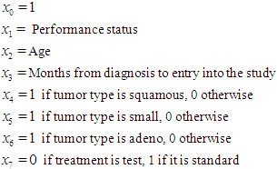 It is wise to center the regressor variables: we have centered just
  here and work with the model for which
 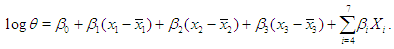 Prior probabilities are specified for regression coefficient
  and shape parameter
  respectively
 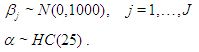 The large variance and small precision indicate a lot of uncertainty of each
  and is hence a weakly informative prior distribution. Similarly, half-Cauchy is weakly informative prior for
  (Statisticat LLC 2014).Model<-function(parm,Data){ ### Parameters beta<-parm[1:Data$J] alpha<-exp(parm[Data$J+1]) ### Log-Prior beta.prior<-sum(dnorm(beta,0,1000, log=TRUE)) alpha.prior<-dhalfcauchy(alpha,25,log=TRUE) ### Log-Likelihood mu<-tcrossprod(Data$X, t(beta)) theta<-exp(mu) z<-log(Data$y)-log(theta) z1<-(exp(z)-1)/exp(z/2) z2<-(exp(z)+1)/exp(z/2) lf<-((1/2)*log(alpha)-log(y)-(z/2)+log(dnorm (sqrt(alpha)*z1))) ls<-log(1-pnorm(sqrt(alpha)*z1)-exp(2*alpha) *pnorm(-sqrt(alpha)*z2)) LL<-(censor*lf+(1-censor)*ls) LL<-sum(LL) ### log-Posterior LP<-LL+beta.prior+alpha.prior Modelout<-list(LP=LP, Dev=-2*LL, Monitor=LP, yhat=mu, parm=parm) return(Modelout) }The Model function contains two arguments, that is, parm and Data, where parm is for the set of parameters, and Data is the list of data. There are two parameters beta and alpha having priors beta.prior and alpha.prior, respectively. The object LL stands for loglikelihood and LP stands for logposterior. The function Model returns the object Modelout, which contains five objects in listed form that includes logposterior LP, deviance Dev, monitoring parameters Monitor, fitted values yhat and estimates of parameters parm.
5.3.3. Initial Values
The function LaplaceApproximation requires a vector of initial values for the parameters. Each initial value is a starting point for the estimation of a parameter. So all the beta parameters have been set equal to zero and the remaining parameter, alpha, has been set equal to log(1), which is zero. The order of the elements of the initial values must match the order of the parameters. Thus, define a vector of initial values Initial.Values<-c(coef(lm(log(y)~x1+x2+x3+x4+x5+x6+x7)), log(1)) For initial values the function GIV (which stands for “Generate Initial Values”) may also be used to randomly generate initial values(Statisticat LLC 2014).
5.3.4. Fitting with Laplace Approximation
To fit the above specified model, the function LaplaceApproximation is used and its results are assigned to objet Fit. Its summary of results are printed by the function print. Fit<-LaplaceApproximation(Model=Model, Initial.Values, Data=MyData, Iterations=500, Method="TR", Samples=1000)print(Fit)
5.3.5. Summarizing Output
The function LaplaceApproximation approximates the posterior density of the fitted model and posterior summaries can be seen in the following tables. Table 2 represents the analytic results using LaplaceApproximation method while Table 3 represents the simulated results using sampling importance resampling method (Akhtar and Khan, 2014a).Table 2. Summary of asymptotic approximation using LaplaceApproximation function with Mode stands for posterior mode, SD for posterior standard deviation and LB, UB are 2.5% and 97.5% quantiles, respectively
 |
| |
|
Table 3. Summary of the simulated results due to sampling importance resampling algorithm using LaplaceApproximation function with Mode stands for posterior mode, SD for posterior standard deviation, MCSE for Monte Carlo standard error, ESS for effective sample size and LB, Median, UB are 2.5%, 50%, 97.5% quantiles, respectively
 |
| |
|
5.4. Fitting with LaplacesDemon
Laplace’s Demon requires a vector of initial values for the parameters. Each initial value will be the starting point for an adaptive chain, or a non- adaptive Markov chain of a parameter. If all initial values are set to zero, then Laplace’s Demon will attempt to optimize the initial values with the LaplaceApproximation function using a resilient backpropagation algorithm. So, it is better to use the last fitted object Fit with the function as.initial.values to get a vector of initial values from the LaplaceApproximation for fitting of LaplacesDemon. Initial values may be generated randomly with the GIV function. Thus, to obtain a vector of initial values the function as.initial.values is used asInitial.Value<-as.initial.values(Fit)Now, the function LaplacesDemon is used to analyze the same data, that is, Lung cancer survival data. This function maximizes the logarithm of unnormalized joint posterior density with MCMC algorithms and provides samples of the marginal posterior distributions, deviation and other monitored variables. FitDemon<-LaplacesDemon(Model, Data=MyData, Initial.Values, Covar=Fit$Covar, Iterations=5000,Status=100,Thinning=10,Algorithm="IM", Specs=list(mu=Fit$Summary1[1:length(Initial.Values), 1])) print(FitDemon) 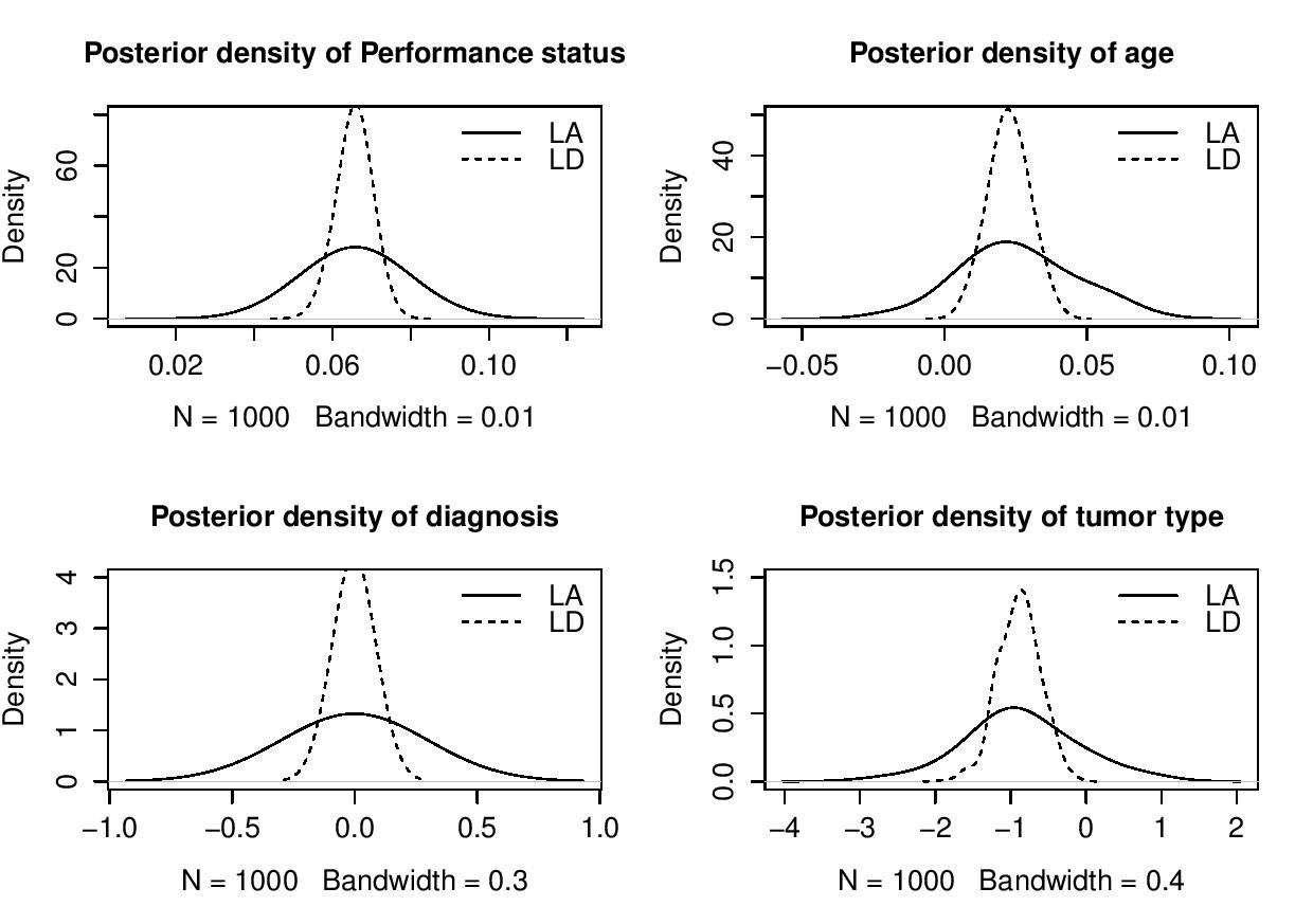 | Figure 3. Posterior density plots of parameters of inverse Gaussian model using the functions LaplaceApproximation and LaplacesDemon |
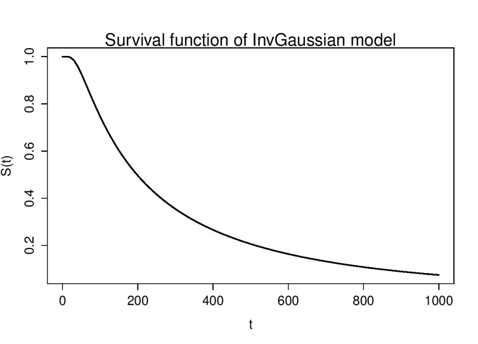 | Figure 4. Survival curve of Inv Gaussian Model |
5.4.1. Summarizing Output
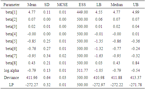
The function LaplacesDemon for this regression model, simulates the data from the posterior density with Independent Metropolis algorithm and summaries of results are reported in the following table.Table 4. Posterior summary of simulation due to stationary samples using the function LaplacesDemon
 |
| |
|
6. Conclusions
The implementation of Inverse Gaussian Distribution as a survival model is presented under Bayesian paradigm. Real life medical data are used for illustrative purposes. The results show that the simulation tools provides better results in terms of standard error as compared to that obtained by asymptotic approximation.
References
| [1] | Akhtar, M. T. and Khan, A. A. (2014a) Bayesian analysis of generalized log-Burr family with R. Springer Plus, 3-185. |
| [2] | Akhtar, M. T. and Khan, A. A. (2014b) Log-logistic Distribution as a Reliability Model: A Bayesian Analysis. American Journal of Mathematics and Statistics, 4(3), 162–170. |
| [3] | Collet, D. (1994) Modelling Survival Data in Medical Research. London: Chapman & Hall. |
| [4] | Collet, D. (2003) Modelling Survival Data in Medical Research, second edition. Chapman & Hall, London. |
| [5] | Gelman, A. and Hill, J. (2007) Data Analysis Using Regression and Multilevel/Hierarchical Models. Cambridge University Press, New York. |
| [6] | Gelman, A. (2008) Scaling Regression Inputs by Dividing by Two Standard Deviations. Statistics in Medicine, 27, 2865–2873. |
| [7] | Lawless, J. F. (1982) Statistical Models and Methods for Lifetime Data. John Wiley & Sons, New York. |
| [8] | Mosteller, F. and Wallace, D. L. (1964) Inference and Disputed Authorship: The Federalist. Reading: Addison-Wesley. |
| [9] | Nocedal, J., and Wright, S. J. (1999) Numerical Optimization. Springer-Verlag. |
| [10] | Meeker, Q. W. and Escobar, A. L. (1998) Statistical Methods for Reliability Data. john Wiley & Sons, New York. |
| [11] | R Core Team (2015) R: A Language and Environment for Statistical Computing. R Foundation for Statistical Computing, Vienna, Austria, ISBN 3-900051-07-0, URL http://www.R-project.org. |
| [12] | Statisticat LLC (2014) LaplacesDemon: Complete environment for Bayesian inference. R package version 3.3.0, http://www.bayesian-inference. com/software. |
| [13] | Tanner, M. A. (1996) Tools for Statistical Inference. Springer-Verlag, New York. |
| [14] | Tierney, L. and Kadane, J. B. (1986): Accurate approximations for posterior moments and marginal densities. Journal of the American Statistical Association, 81, 82-86. |
| [15] | Khan, Y., Akhtar, M. T., Shehla, R. and Khan, A. A. (2015) Bayesian modeling of forestry data with R using optimization and simulation tools. Journal of Applied Analysis and Computation, 5, 38-51. |

 Abstract
 Reference
 Full-Text PDF
 Full-text HTML