1. Introduction

The terrorism became the first security problem in the world. Various and different attack method used by the terrorism such as, suicide attacks by kamikazes, bombs, cars bombs, etc., that their aim is to spread fear, often for the religious or for the ideological purposes [1, 4]. So, the goal of this article is to create a statistical model to prevent the terrorist attacks based on the Self-exciting point process in particular the Hawkes process [2]. The using of this process for several reason; for example, after each attack, the probability of another occurring increased and after reaching a certain point, this increase was decreasing gradually. Another reason to use the self-exciting process is that the correlation are present between nearby events is positive. In the 1971s, Professor Alan Hawkes [3] introduced a family of probability models for the occurrence of series of events. The Hawkes process are a family of point processes. Over the last 15 years their use has spread too many subjects such as, ecology (Whale spotting, spider colonies, invasive banana trees) [13], crime prediction (gang fights, car theft,…), terrorist acts (Iraq, Indonesia) [7], molecular genetics [3], neuroscience; recurrence of cancer tumors, social networks (Twitter, Facebook, YouTube, conversation analysis) [6], finance (Insurance, Credit Risk, Risk Management) [5]. This suggests that the events such as terrorist attacks are not isolated events but are related to each other. It further asserts that the probability of a similar event occurring immediately after decreases as time passes.

We organize this article by different section. In section 2, we describe the descriptive of the terrorist attacks in the world, in section 3, we introduce the point process model, and the standard self-exciting point processes. In section 4, we show the Hawkes process to modeling the attacks terrorism events, then we purpose an inference model to estimate the parameter of the Hawkes process based on the maximum likelihood estimation (MLE). In section 5, we treat a theoretical model to simulate the Hawkes process and we apply the self-exciting process to describe the evolution of the real data in the world and to predict the possible counting attacks terrorism in the future. Finally, we will discuss the conclusion for possible directions for future work.

2. Descriptive of the Terrorist Attacks

The last fifteen years, the terrorist attacks have increased from less than 2,000 to nearly 14,000 [8]. As for the number of deaths, it was multiplied by nine. We have 58% of terrorist attacks committed with bombs and 34% with firearms. The remaining 10% of attacks employ other methods. Between 2000 and 2014, 40% of attacks were committed by unidentified groups. The remaining 60% corresponds to a small number of organizations: Daech, Boko Haram, the Taliban, al-Qaida in Iraq and al-Shabaab are responsible for 35% of the attacks in the world over the last fifteen years. Just between 2013 and 2014, Daesh has implemented 750 terrorist attacks. A recurring element is the targeting of means of transport, especially bus and train (62% of attacks), (see Figure 1) [10].

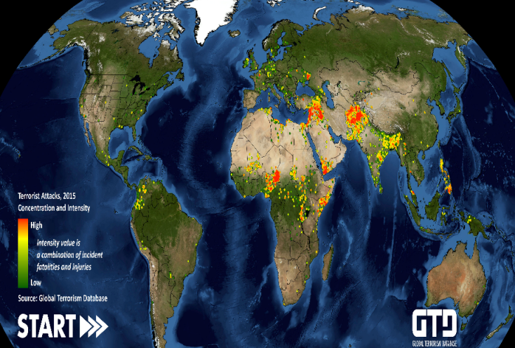Figure 1. Concentration and intensity of the terrorist attacks in 2015 in the world

In 2014 terrorism impacted more countries than ever before. Attacks were recorded in 93 countries, up from 88 in 2013. This continues the trend from 2011 with more countries experiencing terrorist attacks and deaths each year. The flow of foreign fighters into Iraq and Syria continued in 2014 and 2015 [10]. Between 25,000 and 30,000 foreign fighters are estimated to have arrived in Syria and Iraq since 2011; 7,000 in the first six months of 2015. Europe comprises 21 per cent of all foreign fighters, while 50 per cent are from neighboring MENA countries. In the year 2015 the Global Terrorism Index highlights that terrorism continues to rise. For example, the total number of deaths from terrorism in 2014 reached 32,685, constituting an 80 per cent increase from 18,111 the previous year. This is the highest level ever recorded which occurred in the just five countries; Iraq, Nigeria, Afghanistan, Pakistan and Syria, while the terrorism is highly concentrated in a small number of countries, the number of countries which have had a terrorist attack is also increasing (see Figure 2) [10].

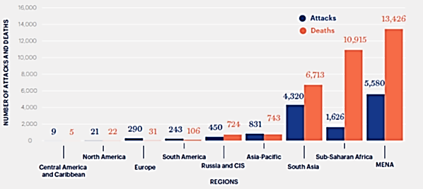Figure 2. Attacks and deaths by region in 2015

We see in the figure 2, the Middle-East and North Africa (MENA) and Sub-Saharan Africa have the highest deaths in 2015. The both regions have many more deaths per attack than other regions.

3. Point Process

The point process is a random collection of events which appears in some space and time. The Poisson process is the preliminary model of a point process where two consecutive events are independent. In other words, a point process is classified as a Poisson process if events occurring at two different times are statistically independent of one another which the characteristics by a single parameter or Poisson intensity. Some examples of certain events, incidence of disease, occurrences of fires, earthquakes, tsunamis [11], [12]. We consider the point process which that takes values on and the occurrences arrival times of each attack terrorism events. We say that a point process is orderly if for any time

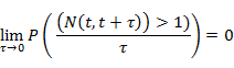A point process is typically characterized by prescribing its conditional intensity , which represents the infinitesimal rate at which events are expected to occur around a particular time given the history of the process up to 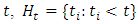(Ogata, 1988) [14], denotes the history of events prior to time

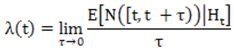Notice that since the right hand side is a conditional expectation, is a random variable. An important example of a point process is the Poisson process. represents the number of events occurring between time and Given disjoint sets 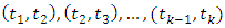where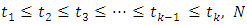 is a Poisson process if the finite dimensional distributions 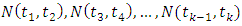each have a Poisson distribution and are independent. Notice that a Poisson process always has a deterministic conditional intensity If the process is stationary then is a constant.

We say that a point process is self-exciting if 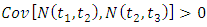for any This means that if an attacks terrorist event occurs, another event becomes more likely to occur locally in time and space. This is not the case for a Poisson process which it has independent increments so . Although Poisson processes have many properties which make them particularly well suited for special purposes, they cannot capture interaction effects between events. So, for this reason we investigate in the next section, a specific class of point process noted a Hawkes Process.

4. Hawkes and Self-exciting Point Process

The Hawkes process is a simple point process, whose intensity function depends on the entire past history and is self-exciting and has the clustering property. The Hawkes process originally states that when an event occurs, it will increase the chance of occurrence of some future events. Over the past few years, Hawkes process models have received significant attentions from researchers, especially in natural phenomena such as seismology research in terms of theoretical and empirical implications. This process can be represented by the conditional intensity function:

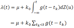(1)

where is the normal counting measure (Hawkes & Oakes, 1974) [15] and is the baseline intensity or the rate of events, denote the points, or event times, of the point process, and is the excitation function. (Zhuang, Ogata, & Vere-Jones, 2002) [16]. The summation describes the self-exciting part of the process with the components and represents the linear dependency over the past events. Many choices for the triggering density have been used (Hawkes, 1971; Ogata, 1988) [3]. In the univariate model of the Hawkes process there is a response function we use an exponential distribution Egesdal et al. (2010) [17] that takes the form of the model (1):

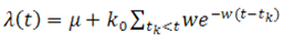(2)

The before the exponential term is the normalization constant. In behavioral terms, corresponds to the strength of the drive to seek retribution for a previous attack, and represents the average time until a repeat event occurs. The intensity function of the univariate Hawkes process in the case of terrorism is usually used to predict the rate of attacks.

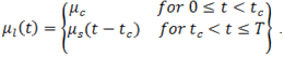
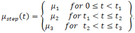
The figure 3 indicates that a stationary background rate is unrealistic for this reason we consider a non-stationary background rate Egesdal et al. (2010) [7], Ogata (1998) [14]. The simplest choice for a non-stationary is a step function parameterized by three values and So we obtain the following model:

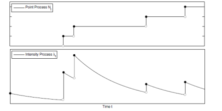Figure 3. Hawkes process with an exponential intensity

(3)

Where

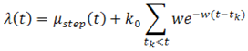
We choose and based on visual inspection of where the largest jumps is occur and we consider the values of and are held constant while fitting the other model parameters.

In this article the number of the attacks terrorist increase, for this we consider another model with a linear rate increase. In this case we obtain the following model:

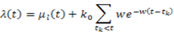(4)

Where

For stationary, it is also assumed that 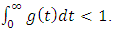By the above specification, we note in particular that the occurrence of an event will make the intensity process jump instantly by the amount which implies an increased chance of another event occurring in a short time interval following the event. This makes the self-exciting process an amenable model for recurrent event data with temporal clustering of events. In applications, two popular choices of the excitation function are the exponential decay function with parameters and the polynomial decay function with parameters and With the corresponding constraints on the parameters, these two forms of the excitation function are both decreasing. From a practical point of view, it seems reasonable to assume that the residual excitation effect due to an individual event wears out and diminishes toward zero as time elapses. However, more specific assumptions, such as the exponential and polynomial forms, for the excitation function are not always justified.

The terrorism attack model is a particular type of marked Hawkes process for modelling the number and the times of any attacks terrorism. We noted by the number of the attack occurring at time The idea behind using the following model is that the terrorism attack is reflected in the fact that every new attack increases the intensity by For this reason the models (1), (2) and (3), (4) can be defined by:

(5)

Where are parameters, and the exponential density distribution is defined by

Equivalently we could define it by its conditional intensity function including both marks and times:

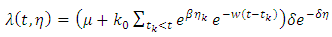(6)

To reduce the risk of model misspecification, it is desirable to leave the form of the excitation function unspecified and estimate it non-parametrically based on the observed data. Based on empirical observation there exist different kernel estimation in the literature, the most widely used are exponential and power law kernel. In this article we use the exponential kernel. There are many methods for parametric estimation of the kernel, such as the Maximum Likelihood Estimation (Ogata, 1998) [14]. We propose the non-parametric estimation model of (Silverman, 1986) [21]. We use variable bandwidth kernel smoothing to construct a smoothed version of the data:

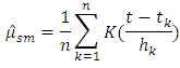Where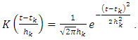

We note by the maximum of the nearest neighbor and by the minimum bandwidth. We know that the rate represent the total of events for this we introduce the parameter So we obtain the following model:

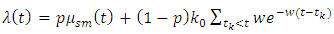(7)

The shape of and is affected by the choices of the nearest neighbor and the bandwidth. To estimate the parameters, we use maximum likelihood estimation [19], [20]. We obtain for the linear model the log likelihood function:

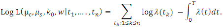We use the Akaike’s Information Criterion (AIC) to compare the models where the 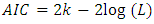[18] where is the number of parameters in the model and is the maximum value of the likelihood function. Egesdal et al. (2010) [17] compare a self-exciting model to a stationary Poisson process with rate equal to the average number of events over the time interval in consideration. In the next section we estimate the parameters of the model by the likelihood method.

5. Inference Model

There exist different method to estimate the parameters in a process specified by a conditional intensity function We apply the maximum likelihood inference or the Bayesian inference which we obtain a simplicity expression of the process. We consider the observed point on an observation interval the likelihood function is given by:

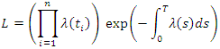Given a marked point 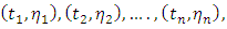the likelihood function becomes:

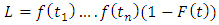
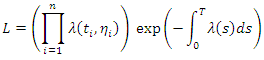By definition, the likelihood function is the joint density of all observed points

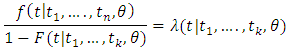
appears since the unobserved next point for example must appear after the end of the observation interval. We assume that the conditional intensity function can be defined by the hazard function:

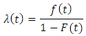And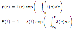

Where is the last point before So we replace and in we obtain:

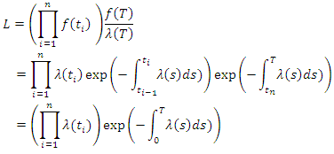Where This result for the unmarked case. To obtain for the marked case, start by the factorization:

Same demonstration in the unmarked case, we obtain:

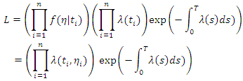Which establishes the result for the marked case.

Given the occurrence observations for an interval 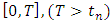the log-likelihood of a point process with an intensity function given in equation (1):

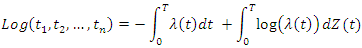Where This is the familiar expression in the case of constant rate. The above log-likelihood is defined under the assumption that the occurrence observations are observed from time to a given time . However in most identification problems, only are given and is not specified. We assume in this article and So the log -likelihood function for the specified intensity function is:

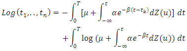Exchanging the variables in the integrals we obtain:

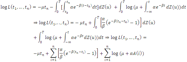Where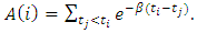

By using the R software we can simulate the hawkes process and the likelihood function in the next section.

6. Simulation and Application to the Real Data

The aim objective of this section is to verify the results of maximum likelihood estimates. The conditional Hazard function:

So,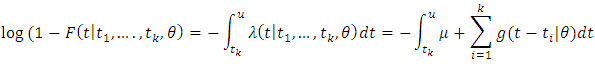

We assume the uniform random variable and we obtain:

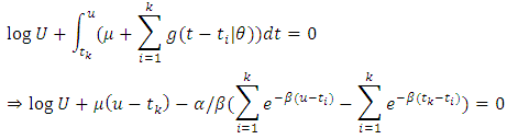Consider the expression in the above equation

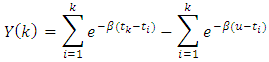This can be written as

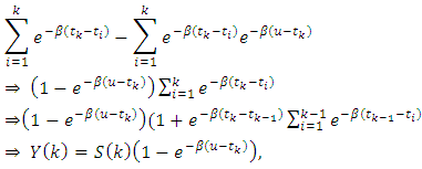With

Hence one can solve the following equation:

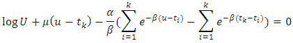And by using the following recursion we obtain:

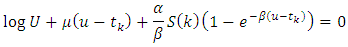Where

And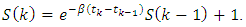

So, based on this recurrence equation we can simulate the Hawkes process with parameters

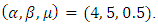The originality of the Hawkes process application is explain in the rest of section. After originally being applied for earthquake prediction it has been also used to anticipate flash crashes in finance, epidemic type of behavior in social media such as Twitter and YouTube or criminality outbursts in big cities. So in this section we apply the Hawkes model to the terrorism events. Our empirical analysis relies on count data drawn from the Global Terrorism Database (GTD) for 1970–2015 [10]. We assume the background rate is stationary, and we compare that process to a stationary Poisson process through the AIC.

The smoothed background rate model outperforms the other models with an AIC value of 801.1. By using the R software to apply Maximum Liklehood Estimator to estimate the parameters for the smoothed background rate model in equation (7), we obtain which means that every event causes between 1 more event on average, and is the average time over which we expect an attack event to happen following a background event, in our case we have days which signifies we have about 17 days to arrive or prepare for another attacks. 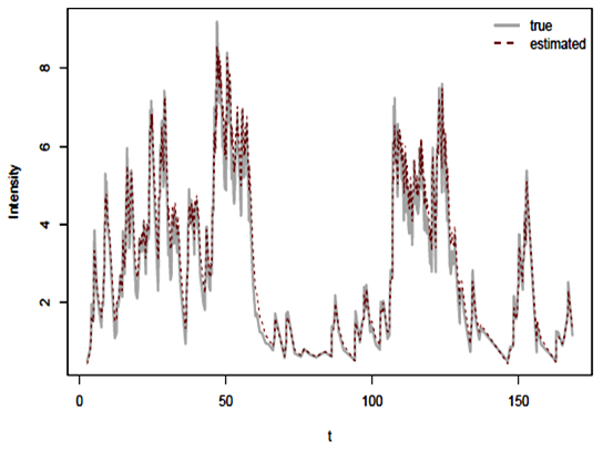We have is equal to the number of events in the interval and 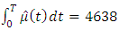is an estimate for the number of background events in the data set which is about 83% of all the attacks terrorism in the MENA region.

Based on Figure 6, we remark the trend form of the data, we remark that the stationary Poisson process is unlikely to give rise to our observed sequence of events. Rather use the AIC to evaluate the self-exciting model against a corresponding non-stationary Poisson model with self-excitation removed 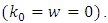We note that the “black’ line represents the initial data set and the “red” line represents the predictive series which we can say the evolution of the terrorism events in the future. By using the SEISMIC software and the dataset (GTD) and the R package we can predict the attack terrorism which that increases the probability that you’ll have another attack which estimate the probability of future attacks at different times and in different areas.

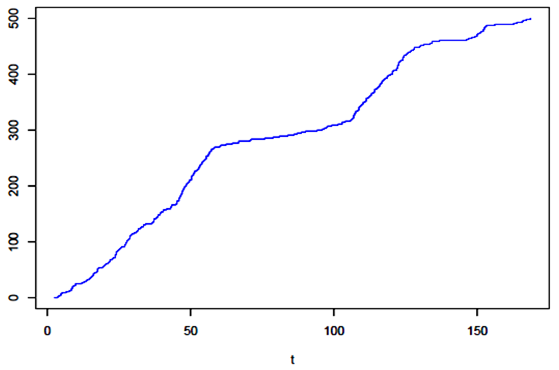Figure 4. Simulated trajectory of the Hawkes process

Figure 5. Estimated intensity function

Figure 6. Terrorism attacks between 1970 and 2015

7. Conclusions

This paper presents the self-exciting model for the analysis and prediction of future terrorist activity. The improvement offered by the self-exciting term provides support for the contagion theory and suggests a significant short term increase in terrorism risk after an attack. The self-exciting hurdle model adheres to the theoretical concept for a contagion effect to terrorism as manifested in the clustering of data while providing good fit and predictive capabilities without relying on exogenous variables. The model provides a simple structure and interpretation of the parameters useful for understanding the dynamic nature of the terrorist activity. This provides an appropriate starting point for exploring additional covariate effects, including analysis concerning the effectiveness of counterterrorism activities, geography, political or economic factors. The utility of the models presented here and their ease of implementation and interpretation make them a potentially useful tool in security related fields. The results show that the risk of terrorist activity can vary greatly over short periods of time, thus policy responses in terms of resource allocation, security and counter-terrorism responses should reflect this as well as addressing the more long-term trends in risk.