C. B. Gupta1, Sachin Kumar1, Brijesh Pratap Singh2
1Department of Mathematics, Birla Institute of Technology and Science, Pilani-Pilani Campus, Rajasthan, India
2Faculty of Commerce & DST-CIMS, Banaras Hindu University, Varanasi, India
Correspondence to: Sachin Kumar, Department of Mathematics, Birla Institute of Technology and Science, Pilani-Pilani Campus, Rajasthan, India.
| Email: |  |
Copyright © 2016 Scientific & Academic Publishing. All Rights Reserved.
This work is licensed under the Creative Commons Attribution International License (CC BY).
http://creativecommons.org/licenses/by/4.0/

Abstract
In the present work, we analysed the distribution pattern of male migrants (aged>=15) from western Utter Pradesh through four basic models viz; Geometric, Poisson-Lindley, Negative Binomial and Zero Adjusted Log Series models. Competency of each of the model was tested with the help of F-ratio test and Vyoung test. A bootstrap test was applied to obtain the size and power of the fitted model. Zero Adjusted Log Series model was found to be the best model to explain the migration behaviour of male migrants of this region.
Keywords:
Migration, Maximum likelihood estimator, Bootstrap, Simulation, and power etc
Cite this paper: C. B. Gupta, Sachin Kumar, Brijesh Pratap Singh, Modelling of Rural-Urban Migration: A Statistical Investigation of Western Uttar Pradesh (India), International Journal of Statistics and Applications, Vol. 6 No. 5, 2016, pp. 293-299. doi: 10.5923/j.statistics.20160605.03.
1. Introduction
Migration has been defined as a permanent or temporary change in residence between some specific defined geographical or political areas. In recent years, it has not only contributed a lot to the change in size and composition of the population, but also it leaves a significant impact on the socio-economic characteristics of the origin and destination population. Rural-urban migration is a flexible and dynamic phenomenon that encompasses territorial mobility of the people and involves movements like commuting, absence from home for periods from a couple of days to several years. It also plays an important role in linking people with spaces and transferring people from a place of lower opportunities to those of higher opportunities. Migration or the movement of people can broadly be classified into two groups (i) long-term migration and (ii) short-term migration. We will focus only on the first type of migration.During the past few decades, many attempts have been made to study the migration process and its impacts ([1], [7], [17], [4], [18]). But the findings of all these methods were based on a macro level approach, which involved a huge set of data from countries, nation, and states as a whole. Therefore, the outcomes of these studies have failed to describe the migration process and pattern, which occurs at the regional and local level. A micro-level approach is needed to clearly explain the mobility behaviour of people. It can be undertaken at the village level, community level or individual level. In almost each and every country, ‘household’ has been accepted as a basic unit to assess the overall socio-economic development of the region. Actually, the number of migrants from a household significantly changes the socio-economic and cultural aspect of the household. It sends remittances, brings new ideas and exposure to the household.Like any other developing country, two types of the household were observed in the study area according to the type of migration. In the first type of households, a male member of family aged 15 years and above migrated singly to other places, leaving their spouses, children and parents at home. They maintained a close contact with their family members left in the village, send remittances and visited the household at a frequent interval of time. In the second type, male members migrated with their spouses, children and other dependent. The characteristics of both types of households are different as far as their socio-economic and cultural impact is concerned. In the first case, there is only male migration, while in the latter, females also migrated. Only the first kind of migration will be studied here.Several attempts have been made in this direction to study the pattern of rural out-migration with the help of suitable probability models. ([14]) were the first, who attempted to propose a Negative Binomial distribution to describe the pattern of this movement at the household level. Later, ([11]) tested the suitability of this model to another set of data and found it unsatisfactory; he proposed the Negative Binomial distribution under certain assumptions, which fitted the data well. ([15]) proposed the mixture of Negative Binomial distribution and Thomson distribution with some assumptions. ([23]) tried to fit the same set of data with inflated Logarithmic distribution. ([22]) introduced the mixture of Poisson distribution and inflated Geometric distribution. They called it as modified Polya-Appelli distribution. But it was suitable for the fitting of a total number of migrants (including females) only. ([16]) proposed a Log Series distribution. But all these proposed models suffered from certain drawbacks. All these models have been proposed and applied to the data taken from eastern Utter Pradesh and Bihar, while our study is based on the data collected from western Utter Pradesh. This part of the state is quite different from the other part, in terms of economic, geographical and social aspects. Higher per capita income, availability of fertile agricultural land, well-developed irrigation facilities and growth of industrial units set this region apart from the eastern Utter Pradesh and makes the region a viable place for migration. To the best of our knowledge, no study has been undertaken in this region to observe the migration pattern of the population involved.Taking the limitations of all these models into account, we have proposed four basic probability models to describe the behaviour pattern of male migrants (aged>=15) from a household. The purpose of this work is, therefore, to compare the applicability of basic statistical distributions to migration data and to provide a set of logical basis to understand the migration pattern clearly. Therefore, our present work has four objectives, to (a) use of Poisson-Lindley, Negative Binomial, Geometric, and Zero Adjusted Log Series models (b) apply the four models to the migration data and to investigate how well these models fit the data (c) comparison of four models and (d) to apply a bootstrap test within a simulation framework to obtain the size and power of the fitted model. To our knowledge, no formal comparison of all these four models has been made to migration data so far.
2. Description of Data
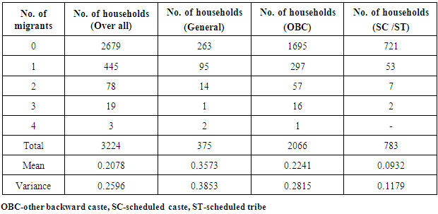
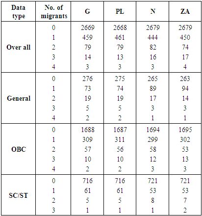
The data used in the present study have been collected from the rural area of district Meerut (U.P.). There has been a rapid spurt of industrial development in and around the city during the past decades and it has become a major hub for various economic, cultural, educational and developmental activities over the years. The baseline survey of nearly 3600 households was undertaken to get the reliable and relevant data pertaining to the problem under study. Following the guidelines from ([13]) data was collected from three types of villages through a stratified clustered sampling method. These three types of the village have been identified as semi-urban, remote and growth centres. We divided the whole of Meerut rural into three regions;(i) Semi-urban areas(ii) Remote areas(iii) Growth centers The villages of Meerut district were classified into two groups according to the distance from Meerut city (boundary of Meerut Nagar Nigam) to form two strata. The villages at a distance of fewer than 8 kilometres formed the first stratum of semi-urban villages, while rest constitute the second stratum called as remote villages. For the selection of growth centres, villages, which were located nearby industrial areas and sugar mills, were taken into consideration. Random selection of 8 and 6 villages was done from these two strata respectively to get approximately 1200 households of each type.All semi-urban villages were put in increasing order of their population size and then divided into three almost equal groups. These groups consist of;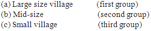 From the first group, with the help of random number table, we selected a two digit random no. and the village corresponding to this no. was selected for the study. The remote village was also put in order of their size and divided in the same way as a semi-urban village.Table 1 displays the frequency distribution of four sets of data, classified according to their category, and shows the number of migrants along with their mean and variances. Each data set shows the variance larger than the mean, a clear indication of over dispersion. One thing is common for each data set that each data set has a peak at no migration and thereafter starts declining rapidly after one migrant, a typical nature of each and every migration data. A minute investigation also reveals a hugely over dispersed nature of the each data set. This might be due to the availability of cultivable land and job opportunities at nearby areas.
Table 1. Frequency distribution of data
 |
| |
|
2.1. Description of Models
(a) Geometric model: let X denote the number of male migrants (aged>=15 years) from the household. It is observed in the survey data that the probability of a number of male migrants decline rapidly i.e. probability of migrating k males from a household is greater than the probability of migrating k+1 males. Therefore, a situation arises when the number of male migrants from the household follows a Geometric distribution. Its mean and variance are given by
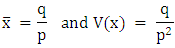 (b) Negative Binomial model: Let X be the number of male migrants aged 15 and above. 14have shown that the number of male migrants from a household follows a negative binomial distribution and probability of exactly K males aged 15 and above is given by;
 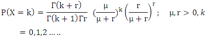 Where µ is the mean number of migrants per household and r denotes the dispersion parameter. The variance of the Negative Binomial distribution is given by
 We can observe that as the value of r increases, so is the over dispersion.(c) Poisson-Lindley model: (i) The number of male migrants aged 15 and above is a random variable and follow a Poisson distribution with parameter λ i.e.
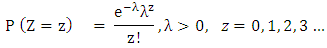 Where Z denotes the number of male migrants aged 15 and above and λ represents the risk parameter.(ii) The risk parameter λ varies from household to household and follows a Lindley distribution proposed by ([8]);
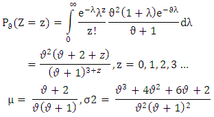 Where ϑ is the parameter of Poisson-Lindley distribution. The variance of Poisson-Lindley distribution is greater than its mean ([3]) i.e. it is over-dispersed, therefore, it can be used for modelling of over- dispersed data.(d) Zero Adjusted Log Series distribution: 6 introduced the ‘logarithmic with zeros’ distribution, later on, which was renamed as Zero Adjusted Log series distribution with the following p.m.f.;
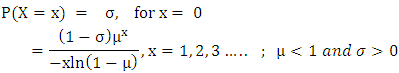 Where σ is the probability that a household is not exposed to the risk of migration, µ is the parameter of log series distribution. Mean of the Zero adjusted log series distribution is given by;
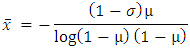 Now equating the observed probability of zeroth cell and mean with its theoretical values i.e.
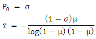 Where
Where  represents the proportion of zeroth cell and observed mean respectively.
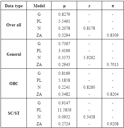
2.2. Parameter Estimates
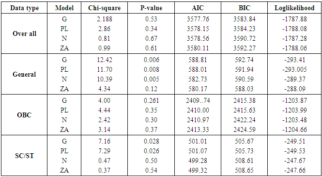
The maximum likelihood estimation (M.L.E.) method was employed to estimate the parameters of the four probability models. M.L.E. was used since this method possesses several desirable properties and advantage over another method of estimation. It is more robust in the sense that it possesses the properties of invariant, asymptotic normality, consistency, sufficiency and minimum variance for large samples. The values of various estimated parameters are shown in table 2. The lower value of r for SC /ST category indicates that this data set is hugely over-dispersed and lower value of φ for general category gives an indication that this category is more prone to migration. The p-value from table 4 also demonstrates that Zero Adjusted Log series distribution provides a good fit across all the categories. Though Geometric, Poisson-Lindley, and Negative Binomial distribution also provide the good fit, but they do not seem to be consistent for each category (table 4). But, when we look at the AIC and BIC, Zero Adjusted Log Series model gives higher values for both AIC and BIC as compared to other models. Table 2. Estimated results of parameter
 |
| |
|
Table 3. Distribution of fitted frequencies
 |
| |
|
Table 4. Goodness of fit measures
 |
| |
|
2.3. Model Accuracy Results
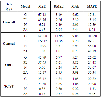
Table 5 displays model accuracy results for all the four models. It is the most popular method of observing the efficiency of the model when several models are in the fray. ([5]) have described several measures of accuracy. Some measures are scale dependent and some are scale independent. Scale-independent measures should not be used across different data sets which are not on the same scale. We have used four following measures of accuracy.Table 5. Comparison of accuracy measures
 |
| |
|
(a) Mean square error (MSE): It is a scale dependent measure of error.MSE = mean (Zi –Ži)2, where Zi is the observed value and Ži is the fitted value.(b) Root mean square error (RMSE): RMSE = √MSE. It has the advantage of being on the same scale as the data, but both MSE and RMSE has the demerit of being more sensitive to the outliers.(c) Mean absolute error (MAE): 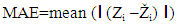 (d) Mean absolute percentage error (MAPE): MAPE has the advantage of being scale dependent, reliable and easy to calculate. It can be used across different data sets, which are on the different scale. The formula for MAPE is given as follows;
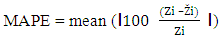 In table 5, accuracy results of all the four measures are given for each data set. The model with the least error is preferred. It is evident from the table that Zero Adjusted Log Series model fits the data with a minimum error for the majority of data sets. Though, Negative Binomial is also very close. Both these model displays a substantial degree of improvement over the other two models i.e. Geometric and Poisson-Lindley distribution.
3. Comparing Models
F-ratio test and Vuong statistic were used to compare the fitted models. F-ratio test is best suited to compare the nested models. In nested models, every model has the same parameter and one model has at least one additional parameter. For example, Geometric and Negative Binomial are the nested models. One model is called the reduced or null model  while the other is called the extended or full model
  ([12]) have described the F-ratio test as;
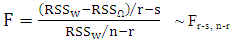
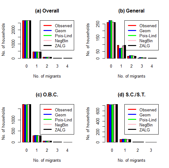 | Figure 1. Observed and expected fitted frequencies from models selected |
Where RSS =∑ (Zi-Ži)2 is the residual sum of squares, r is the number of parameters in the full model, s is the number of parameter in the reduced model and n is the number of observation. It is important to decide which model will act as a null model and be the part of the null hypothesis. One thing to notice, that it is not possible to use F-ratio test where a number of parameters are equal in both the models.Vuong test was proposed by ([20]) to compare the non-nested models. According to this test, let f1(yi/xi) denotes the predicted probability distribution under H0 and f2(yi/xi) is the probability distribution under H1 and let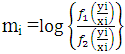 Then Vyong statistic;
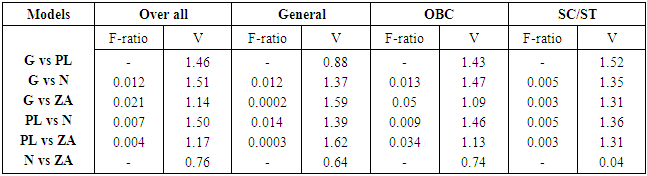
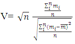 If the value of V statistic is greater than 1.96 then the test favours the full model and if less than -1.96 then it favours the null model. Any value between -1.96 to 1.96 leads to the inconclusive test ([10]).Table 6 demonstrates the p-value of F-ratio test and value of V statistic. The p-value for F-test is less than 0.05 for every combination of models. It means there is a need for a distribution with extra dispersion parameter to handle the over -dispersion in the data i.e. Negative Binomial and Zero Adjusted Log series distribution might give the good fit as compared to Geometric and Poisson-Lindley distribution.
Table 6. Comparison of models
 |
| |
|
4. Simulated Estimates of the Size and Power of the Test to Compare Four Models
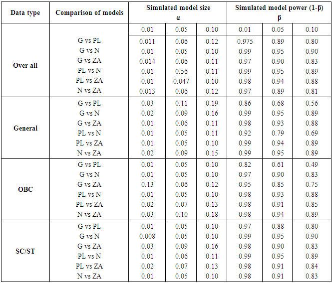
The use of simulation studies, in almost all spheres of science, ranging from aeronautics to health and social sciences, has given an edge to the studies, where real data would not have been possible ([19]). Simulation methods give the empirical estimation of the sampling distribution of parameters involved that was not possible from a single study. ([2]) have provided the detailed procedure and protocol to be followed before any simulation gets started. Simulation technique was used to achieve the estimates of size and power of the test that were obtained from empirical distributions, which were obtained from repetitions of simulated data generated from a particular model. We used a bootstrap approach supported by simulation technique to get the estimate of size and power to compare the competence of the model. Basically, bootstrap is a non-parametric resampling method for estimating sample size, standard error and confidence interval etc. and it involves repeated selection of random samples from the original data with replacement. ([21]) have given a procedure of estimating power and size of the test in detail. P- values were obtained through bootstrapping and then the size of the test was estimated as the proportion of p-values in which the null model was accepted at the actual significance level. The power of the test was computed as the proportion of p-values from each simulated sample, in which we rejected the null model when it is false. All these simulations and bootstrapping were done with the help of R-3.2.2 version ([9]) on a Window 10 platform.All the results from the simulation were summarized in table 7. We used the fitted models based on migration data as to start the simulation process so that the realistic results can be ensured. A number of replications and bootstrap B values varied for each combination of models due to varied dispersion for each model. The bootstrap test gives us the satisfactory results, as is evident from table 7. Though, there was some difference in actual size and estimated the size at some places, when Negative Binomial versus Zero Adjusted model were considered for General and OBC category and Geometric versus Zero Adjusted for SC/ST category. A big gap can be observed across all the data sets in the power when we applied Geometric versus Poisson-Lindley distribution at 0.01, 0.05 and 0.10 level of significance.Table 7. Simulated estimates of the size and power of the test
 |
| |
|
5. Conclusions
From the above study and discussion, it might be concluded that Zero Adjusted Log Series distribution provides a good fit and shows an improvement over Poisson-Lindley, Geometric and Negative Binomial distribution for several sets of data on rural-urban migration of this region. Though Negative Binomial distribution also approximates the good results, but it lacks consistency when applied across all the categories selected in the study. It is observed that a mean number of migrants are higher in General category followed by OBC and SC/ST. The reason behind this phenomenon might be that, usually, General category families are well educated and well informed about the opportunities at other places, so they are more prone to migration. It also reflects the existence of strong joint family culture prevailed in the upper category households of the region. The availability of ample cultivable land, job opportunities in the agriculture farms, brick lin industries, and small scale industries also discourages the single male migration from OBC and SC/ST category households. Given the characteristics of the migration data, our study also confirmed that migration data is over-dispersed, but not because of the heterogeneity of the population.
References
| [1] | Bose A (ed.), Pattern of population change in India, 1951-61, Allied publishers, Bombay, 1-7, 1967. |
| [2] | Burton A, Altman DG, Royston P, Holder RL, 2006, The design of simulation studies in medical statistics. Statistics in Medicine 25: 4279-4292. |
| [3] | Ghitany ME, DK AL-Mutari, 2008, Estimation methods for the discrete Poison-Lindley distribution. Journal of Statistical Computation and Simulation 79:1-9. |
| [4] | Greenwood MJ 1971, A regression analysis of migration to urban areas of less developed countries: The case of India. Journal of Regional Science 11:253-262. |
| [5] | Hyndman RJ, Koehler, AB 2006, Another look at measures of forecast accuracy.Internationa Journal of Forecasting 22: 679-688. |
| [6] | Khatri CG 1961, On the distribution obtained by varying the number of tails in a Binomial distribution. Annals of the Institute of Statistical Mathematics 13: 47-51. |
| [7] | Lansing JB, Muller E 1967, The geographical mobility of labor, Ann. Arbor: Survey Research Centre, University of Michigan. |
| [8] | Lindley DV 1958, Fiducial distributions and Bayes theorem. Journal of Royal Statistical Society, series B, 20: 102-107. |
| [9] | R Core Team 2015, R: A language and environment for statistical computing. R Foundation for Statistical Computing: Vienna, Austria. URL http://www.R-project.org. |
| [10] | Shankar V, Milton J, Mannering F, 1997, Modelling accident frequencies as zero-altered probability: an empirical inquiry. Accident Analysis and Prevention 29:829-837. |
| [11] | Sharma L, 1984, Distribution of number of migrants from a household, Unpublished Ph.D. thesis in Statistics, Banaras Hindu University, Varanasi. |
| [12] | Shen Q, Faraway J, 2004, An F-test for linear models with functional response. Statistica Sinica 14:1239-1257. |
| [13] | Singh RB, 1986, Appendix: Rural Development and Population Growth – A Sample Survey 1978, Unpublished Ph.D. thesis in Statistics, Banaras Hindu University, Varanasi, 130-146. |
| [14] | Singh SN, Yadava KNS, 1981, Trend in rural out-migration. Rural Demography 8: 53-61. |
| [15] | Singh SRJ, 1985, Distribution of number of migrants from a household, Unpublished Ph.D. thesis in Statistics, Banaras Hindu University, Varanasi. |
| [16] | Singh SRJ, 2004, Probability model for the number of rural out-migration. Journal of International Academy of Physical Sciences 8: 31-44. |
| [17] | Speare A (Jr), 1970, Home ownership, life cycle stage, and residential mobility. Demography 7:479-458. |
| [18] | Speare A (Jr), 1971, A cost benefit model of rural to urban migration in Taiwan. Population Studies 25: 117-130. |
| [19] | Vaeth M, Skovlund E, 2004, A simple approach to power and sample size calculations in logistic regression and Cox regression models. Statistics in Medicine 23: 1781-1792. |
| [20] | Vuong QH, 1989, Likelihood ratio test for model selection and non-nested hypotheses, Econometric 57: 307-333. |
| [21] | Walters SJ, Campbell MJ (2005) The use of bootstrap methods for estimating sample size and analysing health-related quality of life outcomes. Statistics in Medicine 24: 1075-1102. |
| [22] | Yadava KNS, Singh KK, Singh RB, 1988, A model for the distribution of distance associated with marriage migration. Journal of Institute of Economic Research 23: 1-12. |
| [23] | Yadava KNS, Singh RB, 1991, A probability model for the distribution of the number of migrants at household level. Genus 47: 49-62. |

 Abstract
 Reference
 Full-Text PDF
 Full-text HTML