S. K. Appiah1, D. Asamoah Owusu1, Edem B. Ahiale2
1Department of Mathematics, College of Science, Kwame Nkrumah University of Science and Technology, Kumasi, Ghana
2Credit Risk Department, Societe Generale Ghana, Accra, Ghana
Correspondence to: S. K. Appiah, Department of Mathematics, College of Science, Kwame Nkrumah University of Science and Technology, Kumasi, Ghana.
| Email: |  |
Copyright © 2016 Scientific & Academic Publishing. All Rights Reserved.
This work is licensed under the Creative Commons Attribution International License (CC BY).
http://creativecommons.org/licenses/by/4.0/

Abstract
The most practical approach to measuring funding liquidity risk in banks is based on the individual bank’s balance sheet (items of assets and liabilities) where inflows and outflows are compared to determine the cumulative cash shortfalls over future time periods. Although steps are then taken to address any resulting funding gaps, the difficulty that the banks face is in assigning future cash flows related to products with indeterminate maturity. The paper presents a non-parametric survival modelling approach to estimating the run-off profile of a bank product with uncertain cash flows. The focus is to contribute to addressing this challenge using the product limit estimator developed by Kaplan and Meier. In view of the subject of the study being in monetary terms, measures are developed to address areas of possible divergence from the normal application of the product limit estimator. The paper then illustrates the framework using a data set from a bank in Ghana to estimate the empirical run-off profile of a savings product over a 30-day period.
Keywords:
Funding liquidity risk, Survival analysis, Kaplan Meier estimate, Products with indeterminate maturity, Run- off profile
Cite this paper: S. K. Appiah, D. Asamoah Owusu, Edem B. Ahiale, A Survival Analysis Approach to Estimating Funding Liquidity Risk in Banks, International Journal of Statistics and Applications, Vol. 6 No. 4, 2016, pp. 259-266. doi: 10.5923/j.statistics.20160604.07.
1. Introduction
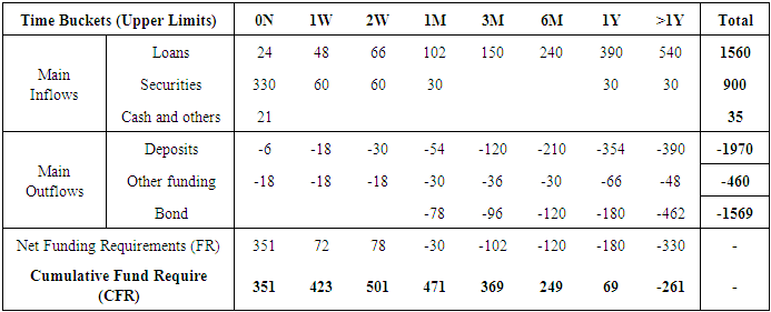
The most popular form of banking in the world is fractional-reserve banking, the practice where banks accept deposits from their customers (surplus units) and extend credit or make loans to other customers in need of funds (deficit units). In this practice, banks need to keep reserves to meet withdrawal requests of depositors (that are usually less than the amounts originally deposited). Most often commercial banks earn little or nothing on reserves; however, being profit seeking entities, the motivation to create credit and earn interest is rife. This means an inherent liquidity imbalance between their assets (typically mid to long term loans and overdrafts) and their liabilities (typically retail deposits and capital market debt). Most of the difficulties experienced by banks at the start of the financial crises in 2007 can be traced to weak liquidity management structures (BIS, 2014 [1]). Ghana had its share of banks going bankrupt even before the global meltdown. In the year 2000, the Government of Ghana and the Central Bank closed down the Bank for Housing and Construction as well as the Corporative Bank due to losses and liquidity issues. The Social Security and National Insurance Trust (SSNIT) had to bail out the Meridian BIAO Bank when it went bankrupt. Funding liquidity risk arises from the liability side for either balance sheet items or contingencies. Banks classify their liabilities on a scale of cash flow certainty, such that items are deemed either stable (core) or volatile. Equity is the most stable although expensive, followed by debt with the secured debt category considered more stable than clean debt. Retail deposits are more stable than wholesale money market deposits. This information is an integral part of cash flow analysis by banks. Banks use several quantitative methods/metrics to measure their liquidity risk including liquidity indices and other peer group comparisons such as borrowed funds/total assets, deposit to loan ratio, funding gaps, stress tests, and liquidity coverage ratio and net stable funding ratio (Basel III) BIS, 2014 [1]). Most practical methods, however, start with forecasting daily inflows and outflows of cash. The process then considers unsecured funding sources and the liquidity characteristics of the asset inventory. Finally, the information is then put together in a strategic perspective. This starts from current assets and liabilities as well as contingencies. The information is used to build a funding matrix. Any gaps should be covered by plans to raise additional funds either through borrowing, disposal of asset or further equity injection (depending on the time). Table 1 shows a hypothetical funding matrix which excludes the off balance sheet items.Table 1. Funding matrix
 |
| |
|
It would appear easy to arrive at a funding matrix if the timing of cash flows associated with the inputs in all instances is known in advance. However, in practice this is not the case. The presence of certain items on a bank’s balance sheet with uncertain cash flow timing presents a forecasting challenge. These items are referred to as non-maturing assets and liabilities (NoMALs) or in other quarters, items having indeterminate maturity. Examples of such items include call deposits and other non-fixed deposit products.The question that needs to be answered is how are banks supposed to measure the run-off rates of products with uncertain cash flow timings? The answer to this question is the main focus of this study. This study aims to extend the boundaries of survival analysis (Lee and Wang, 2003 [2]) to estimating the run-off profile of a bank liability product with uncertain cash flows. It seeks to use observed decrements on a deposit product to obtain an empirical estimate of the distribution function with no prior assumption about the shape or form of its probability distribution.
2. Related Literature
In this section we give a brief review of concepts of funding liquidity risk and its various modelling approaches.
2.1. Liquidity Risk Notions
There are three main liquidity notions, namely, central bank liquidity, market liquidity and funding liquidity (Nikolaou, 2009 [3]). Whilst both the central bank liquidity and market liquidity can be looked at from the macro level, the funding liquidity is more of a micro level phenomenon and generally refers to an entity’s (banks) ability to meet their liabilities, unwind or settle their positions as they become due (BIS, 2000 [4]). The risk will be defined as the probability that the actual realisations of an economic agent will deviate from the expected (Machina and Rothschild, 1987 [5]). Thus, the inability of a bank to service their future obligations as they fall due can be referred to as funding liquidity risk [IMF, 2008 [6]). Banks by virtue of their activity of accepting deposits and granting credit are exposed to this risk. Gauthier et al. (2014) [7] highlights how vulnerable leveraged institutions are to low cash holdings and short term debt.
2.2. Risk Liquidity Modelling
Methods have been developed to address the issue of products with indeterminate maturity. However, available literature is quite varied. Few of such modelling approaches relevant to this study are presented. Bardenhewer (2007) [8] in his study used the replicating portfolio model with embedded options present in savings product. This model was applied to a plain vanilla instruments – money market instruments and bonds, which are actively traded to construct a replicating portfolio deemed to have analogous features such as the timing of cash flows. Another useful technique is by the option adjusted spread models, which are premised on the fact that NoMALs have embedded options in which option pricing theory is applicable to them. Jarrow and van Deventer (1998) [9] provide an approach to compute the present value (PV) of a savings product assuming no arbitrage and complete markets. Time series run off models can also be used to estimate a product with indeterminate maturity’s run-of profile from a statistical distribution (Neu, 2007; Vento and La Ganga 2009) [10], [11]. They focus on the stable portion of NoMALs balance using a log linear time series regression to determine product run off profile at a given confidence level. Kalkbrener and Willing (2004) [12] proposed a stochastic three-factor model for liquidity and interest rate risk management of NoMALs. The account decrements are assumed to follow a normal distribution and used to forecast future account balances. Poorman and Stern (2012) [13] relied on deposit pricing (or asset-liability management) models for estimating liquidity, income, and value metrics among others, and concluded that the life of a deposit follows a Weibull distribution. Using data from South African bank, Musakwa (2013) [14] developed a scenario approach based on survival analysis to measure proportion retained on a savings account product while Matz and Neu (2006) [15] used the proportion of account balances held over time to develop a retention curve. The existing literature on quantitative models for measuring liquidity risk that attempted cash flow timing have mainly inferred run-off profiles of unsecured debt products by studying the time series to show how the position evolved over time and not necessarily the time the product position stayed on the bank’s books (Musakwa, 2013; Neu, 2007; Vento and La Ganga, 2009 [10], [11], [14]). Other studies have tried using other financial instruments to mimic the cash flows inherent in bank savings product (Bardenhewer, 2007 [8]) or adopted estimation methods established for valuing other products (Jarrow and van Deventer, 1998 [9]). There have also been attempts to use a time to event approach but have either assumed a probability distribution for account decrements (Poorman and Stern, 2012 [13]) or rather adopted a scenario based approach (Musakwa, 2013 [14]). This study adopts a simple non-parametric time to event approach to measuring funding liquidity risk and avoids the complexity of a replicating portfolio or scenario based- method.
3. Methodology
The survival analysis modelling for estimating funding liquidity risk (cash flow) in a bank is presented and applied to a case study in Ghana. The study subsequently specifies how the run-off profile can be computed using the product limit estimator (Kaplan and Meier, 19959 [19]).
3.1. Subject of Study
The subject of study is a bank financial product and as such the subjects will be measured in monetary terms. In this case we let a subject of study be 0.01of GHC 1 (GHC is the ISO code for the Ghanaian cedi – implies one-hundredth of a GHC, which is 1 pesewa), such that if  denotes the balance on account
  , then if
  has a balance of GHC 25, then then
 . This similar approach has been adopted by Musakwa (2013) [14]. Let
  be the total amount outstanding (balance) on a savings product at time t and
  be the balance on account
  at time t. Then the two variables are related by:
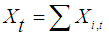 | (1) |
We then define a constantly decreasing function of the total account balances from the start of the trial by: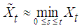 | (2) |
Equation (2) is similar in structure to that of Kalkbrener and Willing (2004) [12] and Musakwa (2013) [14]. However, they differ in their respective uses. The former study used their version of the equation to determine the run-off profile of simulated future account balances, while the later applied it to determine run-off profile on individual account balances. In this study the survival analysis technique (Lee and Wang, 2003; Kaplan and Meier, 1958 [2], [19]) is applied to estimate the proportion of the total outstanding account whose time on the bank’s books exceeds t without imposing a known distribution on the function. It is defined as: 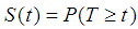 | (3) |
3.2. Suitability of Survival Analysis
Survival analysis relates to data analysis methods that looks at time to the occurrence of some event of interest (Lee and Wang, 2003; Gardiner, 2010 [2], [16]). It is often possible in survival analysis for the event of interest not to be observed in all subjects. These are called censored cases but are still useful as they provide a lower bound for the actual non-observed survival time (Billingham et al., 1999 [17]). The survival function can be estimated using a parametric estimator. In real-life cases, however, a non-parametric method may be appropriate as the actual distribution is usually unknown (Zhao, 2008 [18]). The most commonly used parametric methods include Weibull, exponential and lognormal distributions. The product limit estimator by Kaplan and Meier (1958) [19] is the most commonly used non-parametric estimation method. As indicated by Musakwa (2013) [14], there are similarities between life time modelling and cash flow analysis that allow application of survival analysis to both situations. In both cases the length of time it takes for a subject to remain in a particular state is modelled. Secondly, both cash-flow and lifetime modelling are censored, leading to only partial information on the ’survival’ time to be known for some of the subjects under observation. However, there are areas of divergence – a key difference centres around the time origin to base ’survival’ analysis for cash flow modelling purposes is unclear, unlike the case with lifetime modelling. The method adopted addresses this divergence (see assumptions under the Kaplan-Meier Estimator).
3.3. Kaplan – Meier Estimator
The Kaplan-Meier estimator (also known as the product limit estimator) is widely used in medical studies to estimate patient’s survival rates. It uses information on those who die and those who survive during the trial period and based on a mathematical formula derives estimates of subjects alive at any point in time (Kaplan and Meier, 1958 [19]). Let  denote the ordered times subjects leave a bank’s books via withdrawal. Also, let
  denote the number of subjects leaving the bank’s books via withdrawal and let
  be the corresponding number of subjects remaining (balance) on the bank’s books such that
 etc. Then
 defines the probability of a subject staying on a bank’s book beyond time
  , which is conditionally (depends) on
  , the probability of surviving beyond time
 Also,
Also,  defines the probability of a subject staying on a bank’s book beyond time
 , which conditionally (depends) on
  , the probability of a subject staying on a bank’s book beyond time
  In general, for
 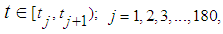 we have (4):
 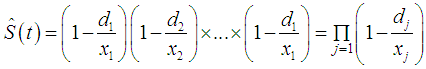 | (4) |
which is the Kaplan-Meier estimator of the survival function 
3.4. Assumptions of the Kaplan Meier Estimator
The key assumptions underlying the product limit estimator are summarized as: (i) There are only two states – the event and censored, which are mutually exclusive. In this study, a case of withdrawal from the account is considered “failure”. Any other case of exit from an account is considered a censored case.(ii) Ability to precisely record event and censorship times is required.(iii) Starting point for the experiment should be clearly defined. Unlike in life experiments where the start date is easy to determine, this study focusses on cash flow modelling using multiple account information. For cash flow modelling using multiple account data, the start date may be different for each account. The analysis is at aggregate level therefore an aggregate level start date is required which will take into consideration as many observations as possible. Let  denote the time origin of subjects in account i from base date b, (which is date in this study is the 180th day as the study covers daily account data over a six-month period). The balance in account i at time
  is denoted
  The start time for account i occurs at
  defined by (5):
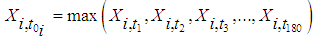 | (5) |
where  represents historical balances on account i from and including the base date and
  With the start time
  for account i, and the corresponding outstanding amount
  at that time now obtained, we let
  be the total number of accounts used in the study such that
 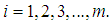 Then the average start time
  which corresponds to the aggregate level start time is
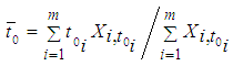 | (6) |
The aim of defining the aggregate level start time from several account start times is to allow for as many observations of the event of interest as possible.(iv) The Kaplan-Meier estimator assumes independence of the subjects of study (Breslow and Crowley, 1974; Gill 1980 [20], [21]). This study also assumes independence of subjects under study. However, with subjects grouped into accounts and such accounts having the same owner; subjects within an account may tend to be correlated. Such correlation is however not expected to result in different estimate of the survival function but rather its variance (Williams, 1995 [22]). It is however safe or reasonable to assume independence in the case of subjects belonging to different account-owners (Musakwa, 2013 [14]).
3.5. Case Study
This section illustrates how to use the theoretical framework developed in section 3.3 to estimate the run-off profile over a 30-day period for deposit product in a bank in Ghana. Simple random sampling was used to select thirty (30) accounts, each representing one branch of the thirty major branches of the bank chosen for the study in the country. Daily account data on deposits, withdrawals, and balances were collected, covering a period of six months (including weekends). This yielded 180-day data set, since as a practice it is expected that even newly established accounts will see some considerable amount of transactions during this period. The data was obtained with the help of staff of the Credit Risk Department of the subject bank.
3.5.1. Aggregate Level Data
The account level data were summed up to obtain aggregate level data across all the 180 days observed using equation (1). That is, the balance on one account on a particular day is added to the balances on other accounts of study for that same day. Similarly, all items of credit and items of debit were added across accounts for each day. The totals on each account were then converted to 1/100th of a monetary unit as defined in section 3.1. Data on credits or increments on the account, though not the subject of this paper, was collected for control purposes to ensure accuracy in account balance data collection. All incidences of censoring were noted during the data collection stage and are separated from event data. Table 2 illustrates the process of data aggregation.Table 2. Aggregate level data at the bank’s branches
 |
| |
|
3.5.2. Aggregate Level Start Time
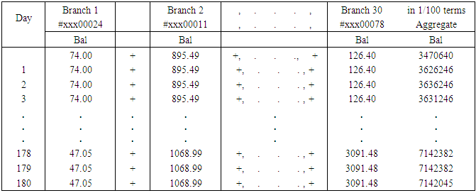
Starting from the base time (180th) and working backwards (using historical data), the maximum balance and the time recorded on each account is obtained. This serves as the starting time for each account in accordance with (5). This is illustrated in Table 3 using accounts from the branches. For example, the first branch recorded its maximum balance of GHC374 on day 50, the second branch recorded its local maxima of GHC1,751 on day 62, and the process continued in this progressive manner until the all the 30 accounts are exhausted. In processing account level start time, it is possible to have in certain situations the maximum balance spanning different time periods or occurring at different times. In such instances the most recent time at which the maximum balance occurs is the most suitable. Figure 1 and Table 3 further illustrate the processes describe above. | Table 3. Accounts’ balances at bank branch level |
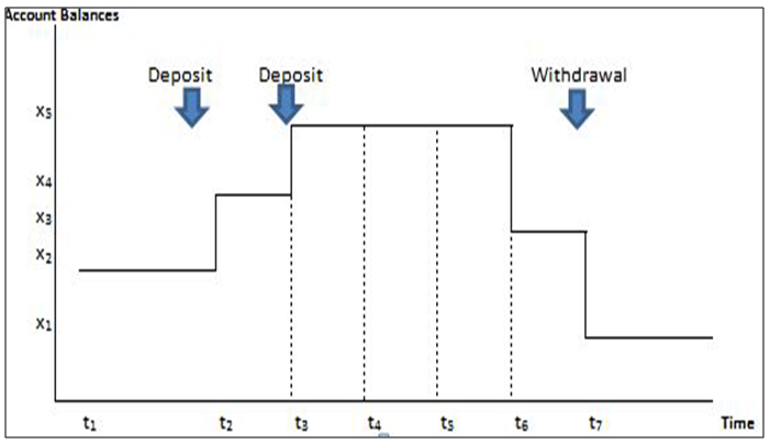 | Figure 1. Individual account starting point (Musakwa, 2013 [14]) |
The weighted average start time using (6) represents the aggregate level start time. From the individual level start times and balances indicated in Table 3 above, the aggregate level start time corresponds to the 89th day. Undoubtedly, this process will be quite strenuous in practice considering the number of individual accounts held at banks. Thus investments in computational power will have to be made. That notwithstanding, inferring the aggregate level start time from individual account start times ensures that more observations of the event of interest - in this case withdrawals - are captured in the estimation process as well as improves the credibility of the process.
4. Results
4.1. Aggregate Level Run-Off Profile
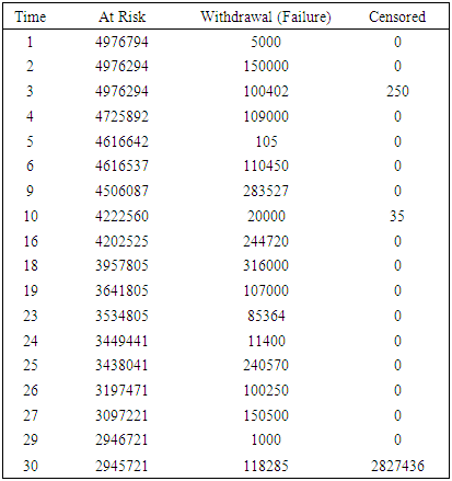
The run-off profile of the savings account product is estimated using the Kaplan-Meier estimator (4) by incorporating the aggregate level start time and the corresponding aggregate level balance (5) as well as decrements over the 30-day period, yielding the survival data in Table 4.Table 4. Survival data
 |
| |
|
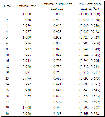
As noted from Table 4, the start time t =1 corresponds to the total individuals account value of 4,976,794 at risk of withdrawal. These gradually reduce as time elapses as signified by the number of withdrawals and censored items. In all, a total of 2,149,073 withdrawals (failures) were recorded during the 30 days of observations while 285 were censored. In addition, a total of 2,827,436 did not record the event of interest (i.e. withdrawal) at the end of the study period and were thus considered censored. In a discrete time framework, as shown in Table 4, censoring times often coincide with the withdrawal times. At such times, this study adopts the convention of assuming that withdrawals precede censoring. Table 5 summarizes the survival distribution function estimation with 95% confidence interval (CI) values while Figure 2 presents the Kaplan-Meier survival curve. The survival curve (solid blue line) which gives the mean estimates of the survival function coincide with either the lower or the upper bound of the CIs (dotted red lines). The mean survival time is estimated at 23.995 with 95% CI of (23.987, 24.003). Table 5. Summarized Kaplan Meier
 |
| |
|
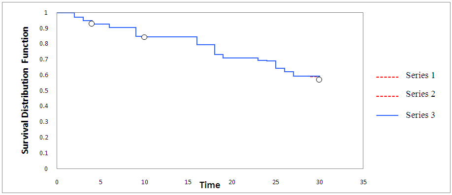 | Figure 2. Kaplan-Meier survival curve estimating the survival function S(t) (solid blue line) with 95% confidence interval (red dotted line’s) |
4.2. Funding Liquidity Risk
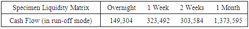
Using the information from the survival curve (Figure 2) and knowledge of proportion withdrawn up to time t = 1 – proportion retained up to time t, a run-off profile equivalent to the estimate of the funding liquidity risk on the deposit product is provided in Table 6 below:Table 6. Specimen of liquidity matrix
 |
| |
|
4.3. Benchmarking
The framework for measuring funding liquidity risk in the subject bank includes among others the following provisions on retail deposits and run-off rates for non-maturing liabilities as illustrated by Figure 3. The stability of the retail and small business centre deposits is determined according to the hierarchy of following criteria (the three stages in Figure 3), which allow classifying the deposits of the customers into stable/less-stable with the above run-off rates – 5% for stable and 10% for less stable:Ÿ Distinguish the guaranteed and not guaranteed deposits insured/guaranteed deposit.Ÿ Detect the transactional accounts transactional account. Ÿ Detect the customers in established relation with the bank.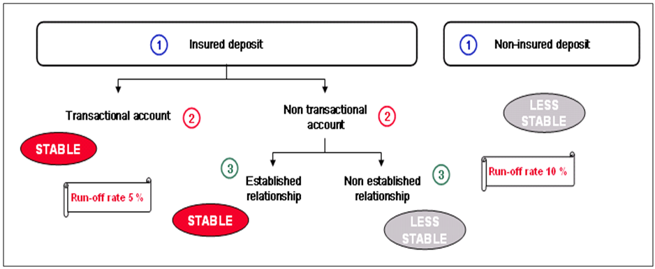 | Figure 3. Measuring funding liquidity by three main stages |
In summary the product limit estimator developed by Kaplan and Meier (1958) [19] was used to estimate the run-off profile of the savings product. The approach developed was illustrated using data from a bank in Ghana over a 30-day period. The individual and aggregate level start time aided in analyzing cash flow timings in a survival analysis context. The findings from the application of the product limit estimator, comparing with the practices of the bank offer evidence to suggest that the current practices by the bank, which uses the Basel III (BIS, 2014 [1]) proposed run-off rates, estimates a much lower funding liquidity risk than the bank assumes. The results of the analysis also show that run-off rates for shorter time buckets are not uniform as regulatory requirements appear to indicate. The overall deposit run-off rate to 30 days stood at 43.2%. For retail and small business centre deposits, internal practice by the bank suggests a maximum run off rate of 10% which is quite low relative to the results achieved via survival analysis.
5. Conclusions
This study has developed a straightforward quantitative framework for measuring funding liquidity risk associated with bank products with indeterminate maturity. Using survival analysis approach the study focussed on determining the run-off profile of a bank deposit savings product. The suitability of applying survival analysis techniques to cash flow modelling was questioned (Musakwa, 2013 [14]). Using the weighted average of individual account starting positions aided in addressing a key area of divergence views between lifetime and cash flow modelling. The technique used in this study also assumed constantly decreasing account balances. This is one of the reasons why a scenario based approach is not adopted as by this assumption. A stress situation had been introduced where during the trial period increments were ignored. This approach is consistent with general risk management practices where adverse but plausible situations are the subject of interest. The framework developed in this paper provides a simple method for estimating the run-off profile for a bank deposit product for managing funding liquidity risk. It minimizes the bias and sophistication introduced by parametric and scenario based approaches. This profile gives the probability of subjects (monetary units) staying in the bank’s books beyond a certain time and aids in addressing the problem of cash flow timing uncertainty when measuring bank funding liquidity risk.The study is however limited by the relatively small number of the sampled accounts used in the analysis and the assumption of independence of intra and inter accounts’ subjects of study. Notwithstanding, the paper contributes to the ongoing debate as to whether Basel III regulator proposed run of rates for both insured and unsecured deposit categories are suitable for implementation. The paper provides grounds for further study in view of its limitations. One possible study to consider is resorting to in-house approach to estimating the run-off profile rather than to proposed standards by the regulator as this presents a more localised approach to dealing with funding liquidity risk. Another area for further study could be estimating the run-off profile of different product classes or business lines (branches) for strategic risk management of individual banks. Further work could also be to model the evolution of a product’s balance by separately projecting the run-off of existing and future business. Lastly, the point on independence of subjects in the same account or across accounts could be explored.
References
| [1] | Bank for International Settlements (BIS) (2014). Basel Committee on Banking Supervision (2014), Paragraph 3. |
| [2] | Lee, E.T. and Wang, J.W (2003). Statistical methods for survival data analysis. 3rd edition. New York: John Wiley & Sons. |
| [3] | Nikolaou, K. (2009). Liquidity (risk) concepts: Definitions and interactions. Working Paper: European Central Bank, Frankfurt, Germany. |
| [4] | Bank for International Settlements (BIS) (2000). Basel Committee on Banking Supervision. Sound practises for managing liquidity in banking organisations. Paragraph 3. |
| [5] | Machina, M.J. and M. Rothschild. (1987). Risk. In: The New Palgrave Dictionary of Economics, J. Eatwell, M. Millgate, and P. Newman (eds), pp.203.5. London, UK: MacMillan. |
| [6] | International Monetary Fund (IMF) (2008). Global financial stability report. Washington DC, USA. |
| [7] | Gauthier, C., Souissi, M. and Liu, X. (2014). “Introducing Funding Liquidity Risk in a Macro Stress-Testing Framework”. International Journal of Central Banking, 10(4), 105-142. |
| [8] | Bardenhewer, M.M. (2007). Modelling non-maturing products. In: Liquidity Risk Measurement and Management, Matz, L. and Neu, P. (eds), Singapore, John Wiley and Sons. |
| [9] | Jarrow, R.A. and van Deventer, D.R. (1998). The arbitrage-free valuation and hedging of demand deposits and credit card loans. Journal of Banking & Finance, 22(3), 249-272. |
| [10] | Neu, P. (2007). Liquidity risk measurement. Liquidity Risk Measurement and Management: A Practitioner’s Guide to Global Best Practices, 15-36. |
| [11] | Vento, G. A. and La Ganga, P. (2009). Bank liquidity risk management and supervision: which lessons from recent market turmoil. Journal of Money, Investment and Banking, 10, 79-126. |
| [12] | Kalkbrener, M. and Willing, J. (2004). Risk management of non-maturing liabilities. Journal of Banking & Finance, 28(7), 1547-1568. |
| [13] | Poorman, F. and Stern, H.S. (2012). A new approach to analyzing core deposit behaviors. Bank Asset/Liability Management, 28(3): 3–5. |
| [14] | Musakwa, F. (2013). Measuring bank funding liquidity risk. Paper presented at Actuarial Society of South Africans 2013 Convention. Sandton Convention Centre. |
| [15] | Matz, L. and Neu, P. (2006). Liquidity Risk: Measurement and Management. Wiley and Sons. |
| [16] | Gardiner, J.C. (2010). Survival analysis: overview of parametric, nonparametric and semi parametric approaches and new developments. In: SAS Global Forum 2010. Statistics and Data Analysis. |
| [17] | Billingham, L.J., Abrams, K.R., and Jones, D.R. (1999). Methods for the analysis of quality-of-life and survival data in health technology assessment. |
| [18] | Zhao, G. (2008). Nonparametric and parametric survival analysis of censored data with possible violation of method assumptions. ProQuest. |
| [19] | Kaplan E. and Meier P. (1958). Nonparametric estimation from incomplete observations. Journal of the American Statistical Association 53:457–481. |
| [20] | Breslow, N.E. and Crowley, J.J. (1974), A large sample study of the life table and the product limit estimates under random censorship. Ann. Statist. 2, 437-453. |
| [21] | Gill, R. D. (1980). Censoring and Stochastic Integrals, Mathematical Centre Tracts 124. Amsterdam: Mathematisch Centrum. Mathematical Reviews (MathSciNet): MR596815 Zentralblatt MATH, 456. |
| [22] | Williams, R.L. (1995). Product-limit survival functions with correlated survival times. Lifetime Data Analysis 1(2): 171-186. |

 Abstract
 Reference
 Full-Text PDF
 Full-text HTML