Zakaria A. Abdel Wahed1, Mohamed S. Abdallah2
1Faculty of Economics & Political Science, Cairo University, Egypt
2Cairo University, Egypt
Correspondence to: Mohamed S. Abdallah, Cairo University, Egypt.
| Email: |  |
Copyright © 2016 Scientific & Academic Publishing. All Rights Reserved.
This work is licensed under the Creative Commons Attribution International License (CC BY).
http://creativecommons.org/licenses/by/4.0/

Abstract
As a consequence of various theoretical developments, and of improvements in computing strategies, restricted maximum likelihood (REML) estimation has become a viable procedure for estimating the variance components in mixed linear models. In this article, the procedure of Xu and Atchley (1996) has been extended in such a way that can be applied to any general linear model. Further, alternative estimator based on empirical Bayes approach has been derived for estimating the random- effects variance components in the light of REML function. Comparison between the proposed estimator and the estimators provided by Xu and Atchley (1996) and Moghtased-Azar et al. (2014) has been computed under unbalanced nested-factorial model with two fixed crossed factorial and one nested random factor. Finally, all the estimators in the vignette are activated by an illustrative example.
Keywords:
Empirical Bayes, Negative Estimates, Nested Factorial Design, Restricted Maximum Likelihood, Simulation Study, Variance Components
Cite this paper: Zakaria A. Abdel Wahed, Mohamed S. Abdallah, A Comparison of Three Different Procedures for Estimating Variance Components, International Journal of Statistics and Applications, Vol. 6 No. 4, 2016, pp. 241-252. doi: 10.5923/j.statistics.20160604.05.
1. Introduction
One of the most traditional methods to estimate the variance components is REML which is quoted by Thompson (1962). The REML approach may lead to massive computations, thus many algorithms were presented over the years to calculate REML estimates. A proper and comprehensive review of these algorithms can be found in Meza (1993) and Matilainen (2014). One of the interesting features of REML is considering the fixed effects as nuisance parameters in order to take into account the implicit degrees of freedom associated with the fixed effects. A competing estimation approach is based on empirical Bayes (EB) principle which, as opposed to REML, considers both the fixed and the random effects as nuisance parameters whereas the variance components are estimated as hyper parameters from the marginal likelihood function which includes only the observed data and the variance components. In this article, an attempt was made to produce a new estimator that merges between the REML method and the EB approach.It is worthwhile to mention that Components of variance estimation can be traced back to the work of astronomer Airy (1861). Since this time remarkable developments and comparisons have taken place on estimation the variance components either from theoretical perspective, empirical view or both. Consequently a plethora of variance components estimation were proposed resulting in extensive publications of books and working papers in this area. A proper survey review for these methods can be found in Sahai (1979), Khuri and Sahai (1985), Khuri (2000) and Sahia and Khurshid (2005). Due to the complexity of the variance components models, it may be intractable to conduct any theoretical comparison among variance components estimators even for the simplest cases of the linear mixed model with unbalanced data. Consequently a number of attempts were performed to study the statistical properties of the variance components estimators using Monte Carlo simulation under different types of models. For instance, based on crossed models: Swallow and Monahan (1984) made a comparison among ANOVA, MLE, REML, and MINQUE methods, Khattree (1998) compared between his proposed non-negative variance components estimator based on simple modification of Henderson's ANOVA method and the original Henderson's ANOVA method, Lee and Khuri (2000) used the Empirical Quantile Dispersion Graph (EQDG) to make a comparison between the ANOVA and ML estimation methods, Subramani (2012) introduced a new procedure to estimate the variance components in the light of MINQUE approach and compared with ANOVA and MINQUE method, and Chen and Wei (2013) derived parametric empirical Bayes estimators and investigated the superiorities of their estimator over ANOVA method. On the other hand, comparisons based on nested models: Sahai (1976) compared among ANOVA, MLE and REML methods, Rao and Hecker (1997) provided a new estimator based on weighted analysis of means (WAM) estimator which utilizes prior information for estimating the variance components, further they compared numerically between their estimator and other traditional variance components methods, Jung et al. (2008) compared between ANOVA and MLE methods based upon the EQDG. Finally El Leithy et al. (2016) suggested a new estimator based on the estimator of Subramani (2012) and made a comparative study between the proposed estimator and other common estimators using nested factorial models with two crossed factors and one nested factor.This article is structured as follows: Section 2 will explain in details the variance component estimator proposed by Moghtased-Azar et al. (2014) which is donated as modified REML (MREML) estimator. In Section 3, the variance component estimator based on EB aspect proposed by Xu and Atchley (1996) will be discussed. A proposed variance component estimator is introduced in Section 4 which is called modified empirical Bayes (MEB) estimator. Section 5 includes the Monte Carlo results using nested-factorial model. Section 6 includes an illustrative application for all the preceding estimators. Finally, some conclusions about this work are given in the last section.
2. MREML Method
Consider the variance components model | (2.1) |
where  is an
is an  vector of observations,
  is an
is an  matrix with known constants,
  is an
is an  vector of fixed (unknown) parameters,
  is an
is an  matrix of known constants and
  is
is  random vector which has multivariate normal distribution with zero mean and covariance matrix
  . Further it is assumed that
  and
and  are uncorrelated. Model (2.1) can be expressed in a compact form as:
 | (2.2) |
where  and
and  . The model (2.2) is called a mixed linear, model. If
  , it becomes a fixed model and if
  it becomes a random model. Thus generally we have
  and
and  , where
  is called the dispersion matrix and the parameters
  are the unknown variance components whose values should be estimated.Since the normality distribution is assumed, thus it is acceptable to operate distribution-based methods. The preferred parametric method for estimating variance components is REML. The original reference to REML is the article by Thompson (1962). Theoretically, REML can be illustrated as assuming
  be a full rank matrix, where
  is the rank of
  , such that
  , 1 then the likelihood of
  can be formulated as:
 | (2.3) |
where  is a vector of the unknown variance components. The log likelihood of
  becomes:
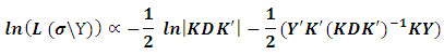 in order to obtain REML estimates, it is required to take the partial derivatives of
  with respect to
  then setting to zero, we obtain
 using the lemma given in Searle et al.(1992) that states:
 hence we will get
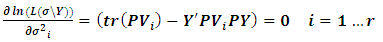 | (2.4) |
It is obvious that we have r equations in r unknowns  . In some cases these equations can be simplified to yield a closed form. Yet, in almost cases numerical algorithms have to be used to solve the equations, it should also be noted that the system of equations in (2.4) does not involve the elements of K, which means no matter what their values are, the same result will be reached (see Searle et al. (1992)). Numerically, Rao and Kleffe (1988) affirmed that REML solutions are equivalent to other variance components estimators (e.g. iterated MINQE, iterated BIQUE and ANOVA) under suitable conditions, weakly consistent, asymptotically efficient and asymptotically normal with zero mean and variance matrix equals to the inverse of the restricted information matrix. Cressie and Lahiri (1993) studied the consistency and asymptotic normality (CAN) of REML estimates in the light of the results reached by sweeting (1980), and applied REML to census undercount in the USA. Jiang (1996) studied the REML estimators in the absence of normality, boundedness of
  and prior specification of the structure of the model. He resorted to deal with REML estimates as a kind of M-estimates in order to reach to the same REML equations. Further, he proved rigorously that the REML estimates are consistent under models that are asymptotically identifiable infinitely and whether the nondegenerate condition is added, then REML estimates are asymptotically normal. Finally, he showed that in the light of the nondegenerate, the REML and ANOVA estimates are consistent and asymptotically normal for all unconfounded balanced mixed models.The main drawback concerning the REML technique is that the solution in (2.4) can be negative, which it is not allowed in the real life. This dilemma has been resolved by Moghtased-Azar et al. (2014). Moghtased-Azar et al. (2014) claimed that using any positive – valued functions can guarantee the non-negativity of the variance components estimates, thus they decided to depend on the exponential function as its range is positive everywhere. Hence obtaining MREML required first to re-parametrize
  as replacing
  with
with  , then maximizing
  with respect to
  instead of
  . After little algebra (2.4) can be reformulated in terms of
  as:
as: | (2.5) |
where 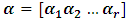 is a vector of the unknown parameters,
  and
and 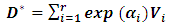 . As explained above, we have r equations in r unknowns
  , solving these nonlinear equations through any iterative algorithm, then the estimated variance components can be calculated by
  . Fortunately Moghtased-Azar et al. (2014) derived an efficient algorithm in order to estimate
  via linearizing (2.5) using Taylor expansion with first order as follows:
  | (2.6) |
where  is the prior value of the
  . The only unknown term in (2.6) is the first derivative of
  which can be obtained as:
 | (2.7) |
After tedious algebra  can be expressed as:
 For simplification, Moghtased-Azar et al. (2014) preferred to deal with
  , which can described as:
  It can easily be proved that:
 hence
hence  will become:
 | (2.8) |
Recall Taylor equation which can be rewritten as: | (2.9) |
where 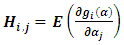 . Consequently getting on MREML based on the following steps:1) Select initial values for
  , in order to calculate
  using (2.5).2) Calculate the
  matrix using (2.8).3) Evaluate
  using (2.9). Then compute
  . 4) Update the initial values in the step (1) with
  evaluated from step (3) and repeat the circle until the convergence achieved. Actually Moghtased-Azar et al. (2014) proved mathematically that MREML is an unbiased estimator and has the same variance as REML, further they showed using an illustrated example that the performance of above algorithm is satisfying and converges quickly.
3. EB Method
In the Bayesian approach, all the parameters are regarded as random in the sense that all uncertainty about them should be expressed in terms of a probability distribution function. The basic paradigm of Bayesian statistics involves a choice of a joint prior distribution of all parameters of interest that could be based on objective evidence or subjective judgment or a combination of both. Generally speaking, the Bayesian approach can be divided into two principal parts. The first one is known as hierarchical Bayesian models which the linear mixed model is considered as a multi-stage hierarchy and all the parameters of the model including variance components should have prior distributions, for more details see Jiang (2007). The second case is known as empirical Bayes or marginal likelihood function that all the nuisance parameters, fixed and random effects, should be integrated out which yields a likelihood function that includes only the observed data and the variance components, thus one can estimate the variance components, as in the classical situations, through maximizing the marginal likelihood with respect to the unknown the variance components (for more details see Searle et al. (1992)). Harville (1977) proved that REML can be considered as an empirical Bayes estimator. He showed that the REML can be derived as the marginal likelihood when the fixed effects are integrated out under a non-informative or flat prior distribution. He used the uniform distribution  , as a prior distribution for the fixed effects
  , however the random effects
  is defined as in (2.1). The marginal likelihood
  can be expressed as:
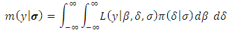 where:
 Since the variance components obtained in (2.4) is equivalent to the variance components obtained using
  , hence the latter suffers also from the negativity problem. Xu and Atchley (1996) proposed a new idea that can be adopted for the estimating non-negative variance components based on empirical Bayes using Monte-Carlo integration algorithm. In this context, the idea will be generalized through the following steps: 1- Express the random effect vector
  as a linear transformation of standard normal deviates which can be expressed as:
  | (3.1) |
2- Use  in (2.3) to derive a new marginal likelihood function in the light of (3.1) as given below:1
  where
where  and
and  .3- Maximize
  with respect to
  , then
  . Which implies that
  is positive under all conditions.Since
  is completely known following standard normal distribution, one can easily generate a huge set of standard normal distribution. Therefore Xu and Atchley (1996) suggested replacing the integrations in
  with the summations to simplify the analysis which yields to:
  One should notice that all
  can be obtained from generating standard normal samples, they stated that as
  , so they recommend to set
  . The maximum likelihood solution of
  required to take the partial derivatives of the
 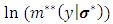 with respect to
  as follows:
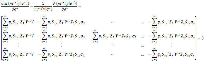 where
where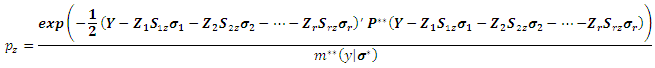 The ML of
  may be written as a linear system by:
 Where
Where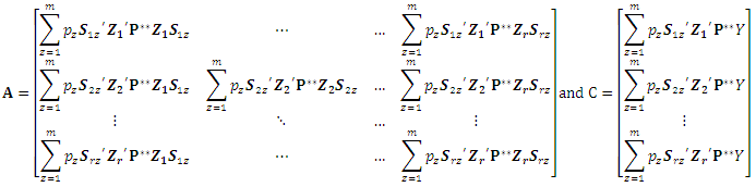 Consequently
  can be calculated as:
  Although algebraically Xu and Atchley (1996) estimator seems to be tedious, it is conceptually very simple, easy to program and avoids inverting large matrix as opposed to MREML estimator which requires to compute the inverse of
  during calculating
  .
.
4. MEB Method
One can derive a new estimator based on EB estimator. Recall that  in terms of
  that can be expressed as:
 Our idea is to solve the above integration analytically, then estimate
  using the algorithm explained in Moghtased-Azar et al. (2014). Fortunately the above integration has explicit form which enables us to obtain MEB as follows:
 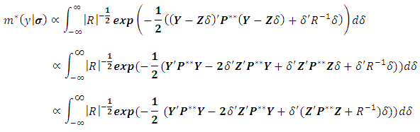 Let us define
 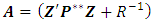 , hence we can get:
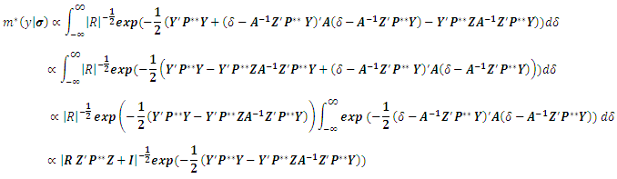 hence
hence 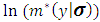 can be presented as:
 Since
Since  is the variance components of
  , thus it can be rewritten as:
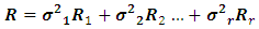 where
where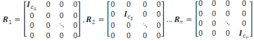 For preventing the negative values of
  , we resort to the idea of Moghtased-Azar et al. (2014) to treat this dilemma as replacing
  with
with  . The maximum likelihood solution of
  required to take the partial derivatives of the
  with respect to
  as follows:
 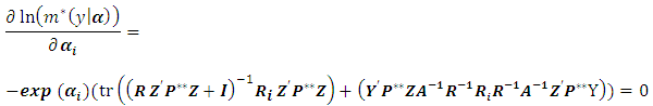 For simplicity we define:
  | (4.1) |
According to (2.6), Taylor expansion with first order may be given as: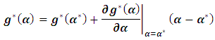 where
where | (4.2) |
The first term in (4.2) can be expressed as: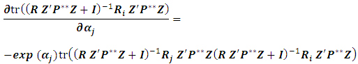 The second term in (4.2) can be derived as:
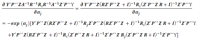 Since the outcome is scalar, hence:
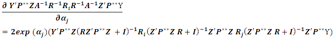 hence
hence  will become:
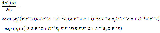 | (4.3) |
Recall Taylor equation which can be rewritten as: | (4.4) |
where  . Consequently steps to get MEB are summarized as following:1) Select initial values for
  , in order to calculate
  using (4.1).2) Calculate the
  matrix using (4.3).3) Evaluate
  using (4.4). Then compute
  . 4) Update the initial values in the step (1) with
  evaluated from step (3) and repeat the circle until the convergence achieved.
5. Simulation Study
Since it may be intractable to do any theoretical comparisons about the performance of the preceding estimators, thus one has to resort to compare through Monte Carlo simulation. Monte Carlo simulation is now a much-used scientific tool for problems that are analytically intractable and for which experimentation is too time-consuming, costly, or impractical. It depends basically on generating artificial random sampling many times, 1000 times for instance, in order to estimate the statistical models and the mathematical functions. Even though, simulation also has disadvantages; it can require huge computing resources, it doesn't give exact solutions, and results are only as good as the model and inputs used.Typically comparisons between the variance components estimators should be conducted under hypothetical model. Following to Melo et al. (2013) and El Leithy et al. (2016), nested factorial design with two crossed factors and one nested factor is adopted in this context in order to identify the behavior of variance components estimators which can be described as:
 , where
  is the effect of the
  level of factor A,
  is the effect of the
  level of factor B,
  is the effect of the
  level of factor C nested within the
  level of A,
  is the interaction effect between the factor A and B,
  is the interaction effect between the factor B and C and
  is a random experimental error. It is assumed that all the effects in the model are fixed parameters except
  are normally independently distributed such that:
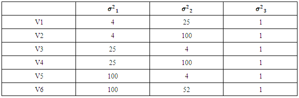
  The main reason for selecting the above model is due to widely usage in the real life, as nested factorial models have the advantage that is suitable for the experiments are either with crossing or nesting factors or both. Since the fixed effects are out of our interest, thus one can fix all the fixed parameters at one. Conversely, the comparison process requires to be conducted under a variety of variance components configurations, difference of imbalance degrees and multiple sample sizes. Following to El Leithy et al. (2016), Table (1). displays the variance components values used in the simulation. The measure which is introduced by Ahrens and Pincus (1981) can be reliable for reflecting the imbalance effect of
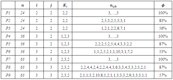
  which can be formulated as:
 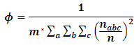 where
where  is the grand sample size and
  is the grand number of the cells obtained by
 , where
  is the levels’ number of the nested factor within the factor
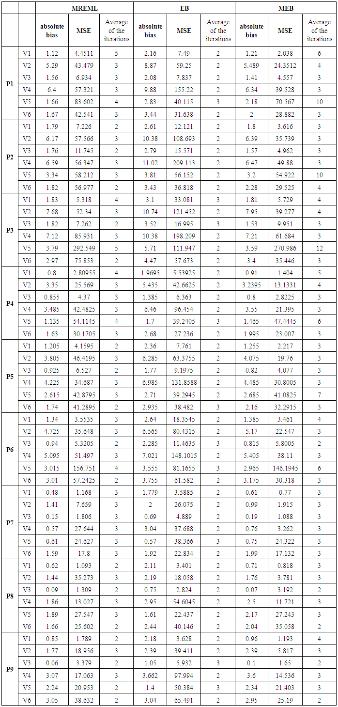
  . Table (2). presents the patterns of imbalance according to different sample sizes throughout the simulation. For each variance components configuration and pattern of imbalance combination, 1000 independent random samples were generated, the estimated bias, MSE and the average of the required iterations for the convergence are shown in Table (3). Since such these estimators are sensitive to the starting points, almost unbiased estimator (AUE) which proposed by Horn et al. (1975) was considered as an initial value in our analysis. The reasons for depending on AUE: 1- Its calculations are simple as it can be expressed in a closed form, 2- It always gives non-negative values. For more details about AUE principle see Searle et al. (1992). According to Table (3), a number of conclusions is drawn from the results for all the patterns and designs which are summarized in the following points:a) It is observed that the three types of the estimators are very close with respect to the number of the iterations particularly at increasing sample size. This result can be explained in light of considering AUE as a primary point which enables the convergence to be achieved rapidly. Generally speaking, EB has the least number of iterations across all the cases.b) It is clear the superiority of MEB over all the estimators in terms of MSE criterion that across almost cases MEB has MSE less than either MREML, EB or both. Whereas MREML estimator has least bias among the preceding estimators. c) The sample size and the imbalance rate have substantial effect on the behavior of all the estimators, as either increasing the small size or reducing the imbalance rate yield a significant improvement in the two measures of the performance. Furthermore, there is an interaction effect between the sample size and the imbalance rate as the effect of the imbalance rate is downward at high level of the sample size.
6. Illustrative Example
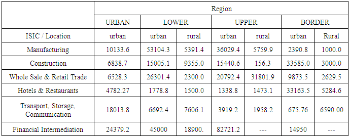
In this part we will just examine the applicability of MREML, EB, and MEB estimators through conducting these estimators on practical case especially large dataset. The application within Information and communication technologies (ICTs) field is provided and conducted via nested factorial model. ICT are used frequently by Private enterprises to improve their productivity and competitiveness in the marketplace. Various kinds of ICT infrastructure such as computer usage, internet usage and mobile usage help firms in all sectors to manage their resources more efficiently. Consequently, it is useful to consider the factors affecting the expenditures of ICT by Private sectors. Accordingly, The Ministry of Communication and Information Technology (MCIT) conducted a survey in 2012 to measure the ICT usage in the private sectors, a proportional sample with size 5,000 enterprises was selected to reflect ICT usage of all Egyptian enterprises. In this context, we will focus only on the ICT expenditures, the location, the region and the International Standard Industrial Classification (ISIC) V.3. of the firms. It is assumed that the ICT expenditures can be mostly affected by the location, the region and the ISIC of the firms. We used the nested factorial design to examine this effect. The raw data are summarized by Table (4) and Figure (1) (see Annex). For the sake of completeness, we write the model equation with the definition of the fixed and random factors in terms of the preceding application as follows:
 , where
  is the dependent variable which is the ICT expenditure for the private sectors after operating the Logarithm transformation two times to guarantee the normality assumption,
  is the effect of the Region factor,
  is the effect of the ISIC factor,
  is the effect of the Location factor nested within the Region factor,
  is the interaction effect between the Region factor and ISIC factor,
  is the interaction effect between the ISIC factor and the Location factor and
  is a random experimental error. Since our sample did not include all ISIC activities, it is assumed that all the effects in the model are fixed parameters except
  are normally independently distributed such that:
  The REML, EB and MEB estimates are calculated for
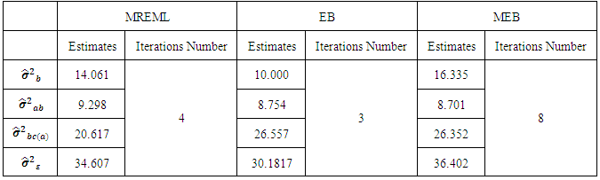
  and
and  and given in Table (5). Since testing hypotheses is beyond the scope of this study, it may interest to take up this topic in the near future.In the light of Table (5), the variance components estimates corresponding to all random factors are estimated by MREML, EB and MEB respectively. As excepted MEB estimator required large number of iterations to converge. In our view, the reason for this point that it is required to simplify equation (4.3) as Moghtased-Azar et al. (2014) done. One can also observe that the
  is relatively large which means that the model needs other factors to explain the variability of the ICT expenditure for the private sectors i.e. the capital size, the number of the employees ..etc. It is easily to remark that since the high degree of unbalancedness of our data, the variance components look somehow different across the studied methods nonetheless the sample size is large.
7. Conclusions
In this article, a new estimator based on empirical Bayes principle is introduced for estimating the variance components in the mixed linear model. The aim of this article is to evaluate the performance of the proposed estimator relative to other two (MREML and EB) estimators via simulation studies. The model we used is the nested-factorial model with two fixed crossed factorial and one nested random factor under regularity assumptions. Three criteria bias, MSE and number of iterations are used to show the performance of all the estimators under the study. From the numerical analysis, we have found that the proposed estimator has desirable properties in terms of MSE, however MREML estimator may be appropriate estimators with respect to bias view, and further EB estimator can be considered as a suitable estimator for handling large data sets since it required low number of iterations to converge.
ACKNOWLEDGMENTS
The authors would like to express their heartiest thanks to the editor and the two referees for careful reading and for their comments which greatly improved the article.
Note
1. Xu and Atchley (1996) discussed multiple marginal likelihood functions, yet we confine ourselves to select which based only on REML.
Annex
Table (1). Variance Components Configurations Used in the Simulation
 |
| |
|
Table (2). The Patterns of Imbalance Rate for Each Sample Size Used in the Simulation
 |
| |
|
Table (3). Comparison of MREML, EB and MEB Estimators Based on Compound Absolute Bias, Compound MSE and Average of the Iterations
 |
| |
|
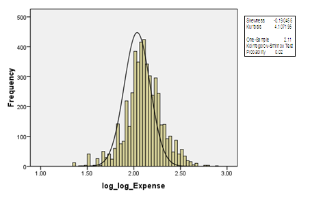 | Figure (1). Histogram of the Logarithm of the Annual Expense with the Normality Test |
Table (4). Average of Annual Expense on ICT for Egyptian Private Enterprises
 |
| |
|
Table (5). Estimates of the Random Factors
 |
| |
|
References
| [1] | Ahrens, H. and Pincus, R. (1981), On Two Measures of Unbalanceness in a One-Way Model and Their Relation to Efficiency. Biometrics.23. 227-235. |
| [2] | Airy, G. B. (1861). On the Algebraical and Numerical Theory of Errors of Observations and the Combinations of Observations. MacMillan, London. |
| [3] | Cressie. N. and Lahiri. S. (1993). The Asymptotic Distribution of REML Estimators. Journal of Multivariate Analysis. 45. 217-233. |
| [4] | Chen. L. and Wei. L. (2013). The Superiorities of Empirical Bayes Estimation of Variance Components in Random Effects Model. Communications in Statistics—Theory and Methods.42:4017-4033. |
| [5] | Diffey .S. Welsh. A. Smith. A. Cullis. B. (2013). A faster and computationally more efficient REML (PX) EM algorithm for linear mixed models. Centre for Statistical & Survey Methodology. Working Paper Series. University of Wollongong. |
| [6] | El Leithy, H. Abdel-Wahed, Z. and Abdullah, M. (2016). On non-negative estimation of variance components in mixed linear models. Journal of Advanced Research. 7. 59-68. |
| [7] | Harville. D. (1977). Maximum-likelihood approaches to variance component estimation and to related problems. JASA.72.320-340. |
| [8] | Horn. S. Horn. R. and Dunca. D. (1975). Estimation Heteroscedastic Variances in Linear Model. JASA.70: 380-385. |
| [9] | Jiang. J. (1996). REML Estimation: Asymptotic Behavior And Related Topics. The Annals of Statistics. 24.1.255-286. |
| [10] | Jiang. J. (2007). Linear and Generalized Linear Mixed Models and Their Applications. Springer Science +Business Media. |
| [11] | Jung. C. Khuri. I. Lee. J. (2008). Comparison of Designs for the Three Folds Nested Random Model. Journal of Applied Statistics.35.701-715. |
| [12] | Khuri. R. (1998). Some practical estimation procedures for variance components. Computational Statistics & Data Analysis. 28. 1-32. |
| [13] | Khuri. A. and Sinha. B. (1998). Statistical Tests for Mixed Linear Models. John Wiley & Sons. New York. |
| [14] | Khuri. A. and Sahai. H. (1985). Variance Components Analysis: A Selective Literature Survey. International Statistical Review. 53. 279-300. |
| [15] | Khuri. A. (2000). Designs for Variance Components Estimation: Past and Present. International Statistical Review.68:311-322. |
| [16] | Lee. J. and Khuri. A. (2000). Quantile Dispersion Graphs for the Comparison of Designs for a Random Two-Way Model. Journal of Statistical Planning and Inference. 91.123-137. |
| [17] | Matilainen. K. (2014). Variance component estimation exploiting Monte Carlo methods and linearization with complex models and large data in animal breeding. Ph.D. thesis. Faculty of Agriculture and Forestry. University of Helsinki. Finland. |
| [18] | Melo. S. Garzón. B. Melo. O. (2013). Cell Means Model for Balanced Factorial Designs with Nested Mixed Factors. Communications in Statistics—Theory and Methods. 42.2009–2024. |
| [19] | Meza. M. (1993). Estimation of Variance Components And Diagnostic Analysis In Unbalanced Mixed Linear Models. Ph.D. Thesis. Texas University. USA. |
| [20] | Moghtased-Azar. K. Tehranchi. R. and Amiri-Simkooei. A. (2014). An Alternative Method for Non-Negative Estimation of Variance Components. Journal Geodesy. 88.427-439. |
| [21] | Qie. W. and Xu. C. (2009). Evaluation of a New Variance Components Estimation Method Modified Henderson’s Method 3 With the Application of Two Way Mixed Model. Department of Economics and Society, Dalarna University College. |
| [22] | Rao. C. and Kleffe. J. (1988). Estimation of Variance Components and Applications. North-Holland, Amsterdam. New York. |
| [23] | Rao. S. Heckler. E. (1997). The Three-Fold Nested Random Effects Model. Journal of Statistical Planning and Inference. 64.341-352. |
| [24] | Sahai, A. (1976). A Comparison of Estimators of Variance Components in the Balanced Three-Stage Nested Random Effects Model Using Mean Squared Error Criterion. JASA. 71. 435-444. |
| [25] | Sahai, A. (1979). Bibliography On Variance Components. International Statistical Review. 47. 177-222. |
| [26] | Sweeting. T. (1980). Uniform Asymptotic Normality of The Maximum Likelihood Estimator. Ann. Statistics. 8. 1375-1381. |
| [27] | Sahai. H. Khurshid. A. (2005). A Bibliography On Variance Components An Introduction And An Update: 1984-2002. Statistica Applicata 17, 191-339. |
| [28] | Searle. S. Casella. G. and McCulloch. C. (1992). Variance Components; John Wiley & Sons. New York. |
| [29] | Subramani. J. (2012). On Modified Minimum Variance Quadratic Unbiased Estimation (MIVQUE) of Variance Components in Mixed Linear Models. Model Assisted Statistics and Applications.7.179-200. |
| [30] | Swallow. H. and Monahan. F. (1984). Monte-Carlo Comparison of ANOVA, MINQUE, REML and ML Estimators of Variance Components. Technometrics. 26.47-57. |
| [31] | Thompson. A. (1962). The Problem of Negative Estimates of Variance Components. The Annals of Mathematical Statistics. 33.273-289. |
| [32] | Wei. L. Ding. X. (2003). On empirical Bayes estimation of variance components in random effects model. Journal of Statistical Planning and Inference. 123.347 – 364. |
| [33] | Xu. S. Atchley. WR. (1996). A Monte-Carlo algorithm for maximum likelihood estimation of variance components. Genetics Selection Evolution, BioMed Central. 28. 329-343. |

 Abstract
 Reference
 Full-Text PDF
 Full-text HTML