O. J. Asemota1, M. A. Bamanga2, O. J. Alaribe1
1Department of Statistics, University of Abuja, Abuja
2Statistics Department, Central Bank of Nigeria, Nigeria
Correspondence to: O. J. Asemota, Department of Statistics, University of Abuja, Abuja.
| Email: |  |
Copyright © 2016 Scientific & Academic Publishing. All Rights Reserved.
This work is licensed under the Creative Commons Attribution International License (CC BY).
http://creativecommons.org/licenses/by/4.0/

Abstract
The modelling of seasonal behaviour of rainfall has become very important in the wake of the climatic change. Due to the agriculture base of the Northeast Nigeria, it is imperative to explicitly model seasonal behaviour of rainfall in the region for agricultural planning. Hence, this study examines the seasonal behaviour of monthly rainfall data from 1981 to 2013 in Maiduguri and Damaturu areas of Borno and Yobe States respectively, using the state space approach. We employed the local level model with stochastic seasonal and the local level model with deterministic seasonal to modelling of the dynamic features in the data. Our results clearly indicate that the local level model with deterministic seasonal is the parsimonious model between the two state space models considered in this study. This implies that the seasonal patterns of rainfall in the two areas have not significantly changed despite the challenges of global warming and climate change. In addition, the CUSUM test indicates the presence of structural breaks in 1998 and 1990 for Maiduguri and Damaturu respectively. This implies that there was an abrupt change in the rainfall level in 1998 for Maiduguri and in 1990 for Damaturu. We, therefore, recommend that seasonality should be explicitly included in the modelling of rainfall series as the pattern of seasonality could be useful for important decision making. In addition, measures should be put in place to curb human-made activities that are detrimental to the climate since the region is highly vulnerable to the impacts of climate change.
Keywords:
Rainfall, Climate Change, Kalman filter, Kalman Smoothing, Seasonality, State space model
Cite this paper: O. J. Asemota, M. A. Bamanga, O. J. Alaribe, Modelling Seasonal Behaviour of Rainfall in Northeast Nigeria. A State Space Approach, International Journal of Statistics and Applications, Vol. 6 No. 4, 2016, pp. 203-222. doi: 10.5923/j.statistics.20160604.02.
1. Introduction
Agriculture in North-Eastern region of Nigeria is predominantly dependent on rainfall. Hence, the output from the sector each year is largely determined by the rainfall seasonal pattern, trend and cycles. Weather as we know is dynamic. Similarly, climate fluctuates or changes over time and space. According to Nieuwolt (1982), the non-static behaviour in rainfall patterns are in various magnitudes ranging from variability through fluctuations, trends, and abrupt to gradual changes. Some characteristics of rainfall which include its seasonal and diurnal distribution, intensity, duration, onset, cessation and frequency of rain days all show important variations in respect to time and places. It is therefore important to examine climatic data to ascertain possible trends and changes in the data generating process. Trend could reflect either an increase or decrease in the observed phenomenon and may serve as a good indicator for predicting future occurrence. A fair knowledge of the weather is very necessary, in view of the fact that farmers, power generation (hydroelectric power generation), meteorological stations, military operations, safety and emergency agencies such as National Emergency Management Agency (NEMA) heavily rely on it for their operations, among other socioeconomic activities. The high amounts of rainfall which are particularly received in many elevated area of the tropics, constitute a reliable basis for the construction of many hydro-electric power stations.There has always been a good deal of interest in the possibility of seasonality in rainfall data. Harvey (1987) pointed out that the analysis of climatic time series is essential for building statistical models to generate synthetic hydrologic records, to forecast hydrologic events, to detect intrinsic stochastic or deterministic characteristics of hydrologic variables. Assessing the seasonal behaviour of rainfall characteristics and trend is a vital for agricultural practice in the North-East states of Nigeria. In addition, the time series analysis of climatic data provides a basis for ascertaining climate change or variability.The Box-Jenkins SARIMA model has been extensively used to model rainfall patterns in Nigeria, see for example, Gulumbe (2013), Etuk, Moffat and Chims (2013) and Martins et al. (2014). However, the Box-Jenkins approach is based on the elimination of trend and seasonality applying seasonal differencing to the series before fitting an appropriate ARMA model to the data. Durbin and Koopman (2001) noted that elimination of trend and seasonality by differencing may pose a problem in applications where knowledge of the seasonal pattern is needed. Fortunately, modern control and system theory has shown that the behaviour of dynamic systems can be conveniently and succinctly described by using the state space models. State space method is more general and is based on the modelling of all the observed features of the data. The different features inherent in a series such as trend, seasonal, cycle, explanatory variables and interventions can be modelled separately before being put together in the state space model. The assumption of stationarity is not needed in state space model.Although the literature on state space has increased recently, there is however, no empirical application to modelling rainfall pattern in Nigeria. In addition, using the state space approach, the nature of seasonality present in the data will be explicitly determined. It is against these backdrops that this study is being proposed. The rainfall received at the synoptic stations at Maiduguri and Damaturu for thirty-three years period (1981-2013) are analyzed to evaluate the seasonal behaviour and trend in the monthly data rainfall. The research is useful in assessing the seasonal behaviour of rainfall characteristics and the trend in the rainfall data which is a vital requirement for agricultural practice in the North-East states of Nigeria. It is also intended to provide a basis for ascertaining climate change or variability. The rest of this paper is organized as follows. In section 2, state space models are briefly introduced, in section 3, we discuss the modelling methodology employed in this work. The data and the empirical results are presented and discussed in chapter 4. The final section concludes the paper.
2. The Model
2.1. State Space Model
A state space model consists of two equations: the state equation (also called transition or system equation) and the observation equation (also called measurement equation). The observation equation expresses the observed variables (data) as a linear function of the state variable(s) plus noise, while the transition equation describes the evolution of the state variables. The transition equation has the form of a first-order difference equation. The selection of components to include in the state space model is based on the features inherent in the observed time series. For a series that have seasonal patterns, the basic structural model is used, for a strongly trending non-seasonal series; the local trend model is employed. However, for a non-trending series, the local level model is used. Let  denote an (n×1) vectors of variables observed at time t and
  be (r×1) unobserved state vector. The general state space representation of the dynamics of y is given by:
 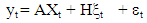 | (1) |
 | (2) |
The (n x 1) vector  and the (k x 1) vector
 are white noise:
  | (3) |
 | (4) |
The disturbances are assumed to be uncorrelated at all lags, that is;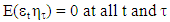 | (5) |
where  is k x 1 vector of unobserved state variables, H is an n x k matrix that links the observed vector
  to the unobserved
  Xt is an r x 1 vector of exogenous or predetermined observed variables, A is a matrix that maps the exogenous variables into the measurement domain, F is the state transition matrix which applies the effect of each state parameter at time t on the system state at time t+1, R is (n x n) and Q is (k x k) matrices of the measurement equation variance and transition equation variance respectively. The R variance matrices play the same role as in the classical regression model, while the Q variance matrices allow the parameters in the state equations to evolve over time. Equation (1) is known as the observation equation and (2) is known as the state equation. The system of (1) through (5) is called state space models. The essential difference between the state space model and the conventional ARIMA model representation is that in the former, the state of nature – analogous to the regression coefficients of the latter – is not assumed to be constant but may change with time.
3. Modelling Methodologies
3.1. State Space Approach: Local Level Model with Seasonality
The local level model or random walk-plus-noise model is a simple form of a linear Gaussian state space model for modelling series with no visible trend. The model contains only the level and irregular components; the single state (level) variable follows the random walk: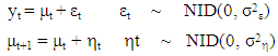 | (6) |
where  and
and  are mutually uncorrelated white-noise processes with variance
  and
and  The interpretation of this model is that
  is an (unobservable) local level or mean for the process. The observable
  is the underlying process mean contaminated with the measurement error εt. Although it has a simple form, it provides the basis for the analysis of important real problems in practical time series analysis. It exhibits the characteristics structure of state space models in which there is a series of unobserved values
  which represents the development over time of the system under study, together with a set of observations
  The aim of the analysis is to study the development of the state over time using the observed values
  However, when a time series consists of daily, monthly, or quarterly observations, the presence of seasonal effects should be taken into consideration. In the state space framework, seasonality can be handled by building the seasonal effects directly into the model. Hence, adding seasonal components to equation above yields,
  | (7) |
where  When the seasonal effect
  is not allowed to change over time, we require
  for all
  This is done by setting
  and (7) is called the local level with deterministic seasonal model. When the seasonal effect
  is allowed to vary over time, that is
  the resulting model is called the local level with stochastic seasonal model. Since the rainfall data consists of monthly observations, the periodicity of the seasonal is s =12. The stochastic formulation of the seasonal effect in (7) follows from the standard dummy variable methods of modelling seasonal pattern. An alternative way of modelling seasonal effect is by using trigonometric terms at the seasonal frequencies. State space models are estimated using the Kalman filter. The Kalman filter is a statistical algorithm that enables certain computations to be carried out for a model cast in state space form. However, to obtain a more accurate estimate of the state vector, the smoothing algorithm is performed. Kalman smoothing provides us with a more accurate inference on
  since it uses more information than the filtering. Let
  denote the set of past observations
  and assuming the conditional distribution of
  given
given 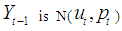 where
where  and
and  are to be determined. Assuming that
  and
and  have been determined, the celebrated Kalman filter equations for updating the above local level model from time
  to
to  are given by:
 | (8) |
for  where
where  denotes the Kalman filter residual or prediction errors,
  is its variance and
  is the Kalman gain. A random walk like
  has no “natural” level and to handle the initial conditions
  for the non-stationary model, we employed the exact initial Kalman filter, (Durbin and Koopman, 2001). The Kalman smoothed state
  and smoothed state variance
  can be calculated by the following backward recursions:
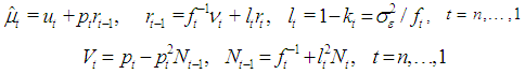 | (9) |
with  and
and  for
for  The unknown variance parameters in the state space model are estimated by the maximum likelihood estimation via the Kalman filter prediction error decomposition initialized with the exact initial Kalman filter. Harvey and Peters (1990) suggested concentration of the log likelihood when the variance parameters display difficult estimation problems, as this helps to improve the behavior of difficult estimation.Diagnostic checking in the state space models are based on the three assumptions concerning the residuals of the analysis. The residuals should satisfy these three properties, in order of importance; independence, homoscedasticity and normality. These assumptions are checked using the following test statistic; The assumption of independence of the residuals can be checked with the Ljung-Box statistic defined as;
 | (10) |
For lags  The number of diffuse initial state values which need to be estimated for the level and seasonal components in (7) corresponds to
  denotes the residual autocorrelation for lag l and w is the number of hyperparameters (i.e. disturbance variances). The second most important assumption is the homoscedasticity of the residuals. This is checked using the following test statistic;
 | (11) |
where d is the number of diffuse initial elements, and h is the nearest integer to (n- d) /3. The least important assumption is that the residuals are normally distributed. This assumption can be checked with the following test statistic;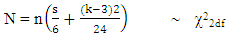 | (12) |
where s denotes the skewness of the residuals, and k is the kurtosis. In the state space models, the standardized smoothed disturbances are useful for detection of possible outliers and structural breaks. The detection of structural break using the cumulative sum (CUSUM) test is considered in this work.
4. Data and Empirical Results
4.1. The Data
The monthly rainfall data for two North-Eastern areas (Maiduguri and Yobe, see Annexure I) from January, 1981 to December 2013 are examined in this study. The monthly rainfall data measured in millimeter is obtained from the Nigeria Meteorological Agency (NIMET), Lagos state office. The plots of the rainfall series are presented in Figure 1 and Figure 2 for Maiduguri and Damaturu respectively.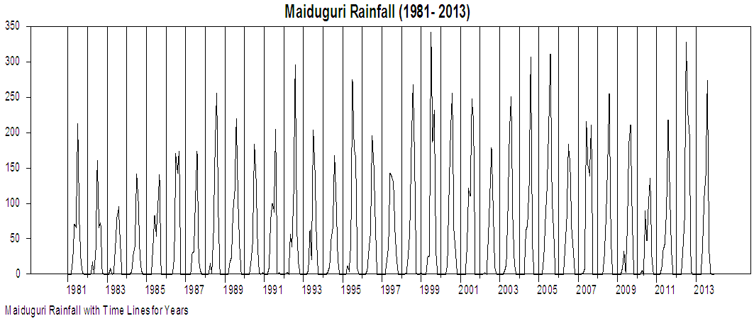 | Figure 1. Time Series Plot of Maiduguri Rainfall |
 | Figure 2. Time Series Plot of Damaturu Rainfall |
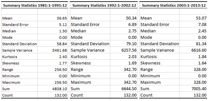
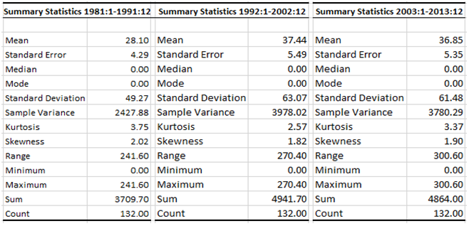
From figure 1 the rainfall series fluctuates over the years but had the highest spike in 1999 and the lowest in 1983 and figure 2 also indicates that the rainfall had its peak in 2012 and the lowest in 1983. The descriptive statistics of the subsamples of both series are presented in table 1 and 2. Table 1 and 2 indicate that the subsample means and variance are not the same over time, which is an indication that the subsample means and variance are not constant. For example, the subsample mean for Damaturu between 1981:1 to 1991:1 is 28.10 while for 1992:1 to 2001:1 and 2002: 1 to 2013:12 are 37.44 and 36.85 respectively. Hence, the means varies across the samples. Thus, the state space model that accommodates non-stationary features by representing the level of the series as a random walk process, since random walk process is non-stationary, would be appropriate for modelling the series.Table 1. Descriptive Statistics of Maiduguri Rainfall
 |
| |
|
Table 2. Descriptive Statistics of Damaturu Rainfall
 |
| |
|
4.2. Estimation Results and Discussion
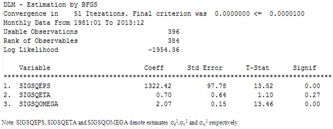
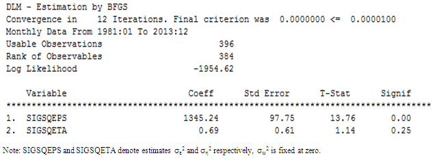
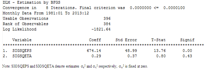
The selection of components to be included in a state space model is based on the characteristics of the observed series. Since seasonality is normally present in a monthly time series data, we employed the local level with stochastic seasonal and local level with deterministic seasonal models described in section 3 to the Maiduguri and Damaturu original series. First, using the data, we estimate the unknown variance parameters (hyperparameters) of the models using maximum likelihood method. This is maximized using the BFGS (Broyden-Fletcher-Goldfarb-Shannon) optimization method. The estimation results for the local level model with stochastic seasonal is presented below.Table 3. Estimation Variance for Local Level Model with Stochastic Seasonal for Maiduguri Rainfall series (1981:1 – 2013:12)
 |
| |
|
Table 4. Estimation Variance for Local Level Model with Stochastic Seasonal for Damaturu Rainfall series (1981:1 – 2013:12)
 |
| |
|
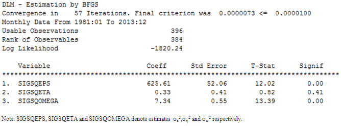
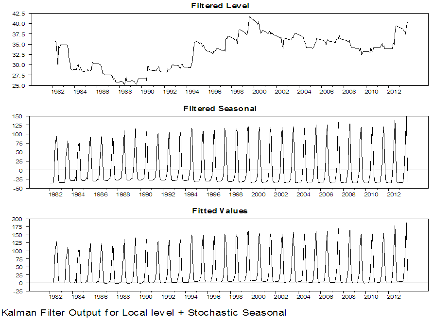
The estimation results in table 3 and 4 indicates that the hyperparameters (disturbance variances) of the measurement and seasonal component are highly statistically significant; however, the estimated hyperparameters for the level equations is not statistically significant. This indicates that any seasonal pattern in the observed time series changes over the years. Also, there are 396 observations in both series; however, the estimation is done using only the final 384 observations. This is because 12 diffuse initial state values are estimated (11 for the seasonal components and 1 for the local level components). We proceed into performing the Kalman filtering and kalman smoothing using the estimated hyperparameters. The results of the Kalman filter estimates for Maiduguri rainfall series is presented in figure 3 and 4 while figure 5 and 6 present that of Damaturu rainfall series respectively.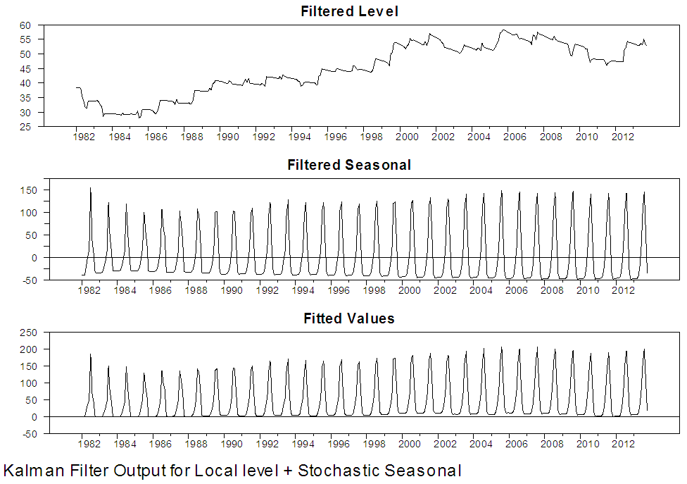 | Figure 3. Kalman Filter Output for local level with stochastic seasonal for Maiduguri series |
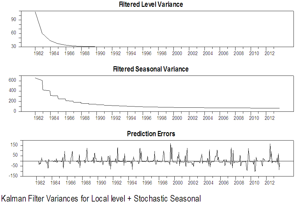 | Figure 4. Kalman Filter Output for local level with stochastic seasonal for Maiduguri series |
 | Figure 5. Kalman Filter Output for local level with stochastic seasonal for Damaturu series |
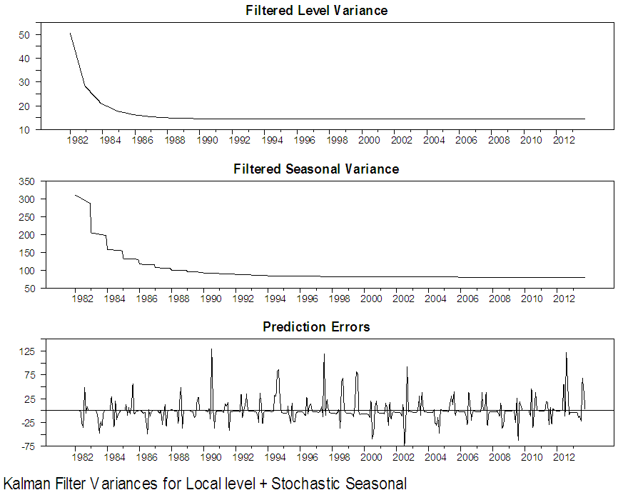 | Figure 6. Kalman Filter Output for local level with stochastic seasonal for Damaturu series |
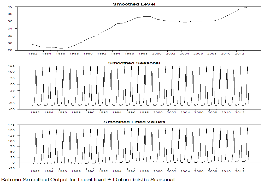
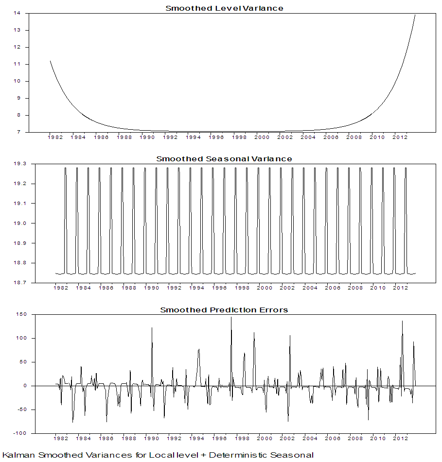
Figure 3 to 6 present graphically the dynamic evolution of the level, seasonal components and the fitted values obtained by the Kalman filter together with their variances and the prediction errors (residuals). The evolution of the two North-Eastern regions under study is reflected by the estimated level component and is presented in the upper graph of figure 3 and 5. The plots indicate that the period of highest level of rainfall in Maiduguri occurred in the 2006 and the lowest level of rainfall occurred in the 1986. From figure 5, the plot also indicates that the period of the highest level of rainfall in Damaturu occurred in the 2000, while the lowest level of rainfall occurred between 1988 and 1989. One obvious features of figure 4 is that, the Kalman filtered state variances converges to zero value, which implies that there is no variability, while in figure 6, the Kalman filtered state variance converges to a constant value as the sample size increases which empirically confirms that the fitted local level model has a steady state solution.Figure 7 to 10 present the results of the Kalman smoothing recursion estimates of the level, seasonal and the fitted values of the series together with the state variances of the level, seasonal component and the smoothed prediction errors respectively. On comparing the graphs of the Kalman filtered level and the smoothed level of the two Northeast states in figure 3 to 5 and 7 to 9 respectively, it is obvious that figure 7 to 9 is smoother than that of figure 3 to 5. In addition, figure 7 to 9 reveal that the seasonal pattern in the Maiduguri and Damaturu series have been relatively constant over the years.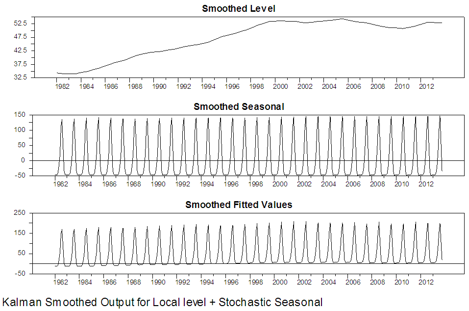 | Figure 7. Kalman Smoothed Output for local level with stochastic seasonal for Maiduguri series |
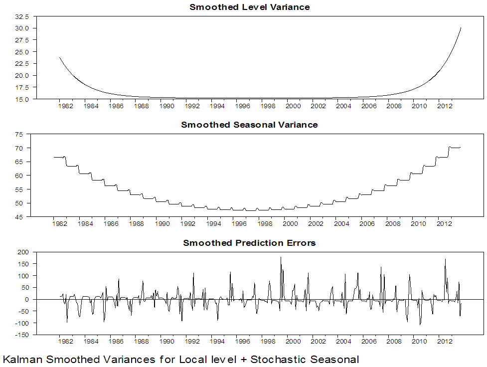 | Figure 8. Kalman Smoothed Output for local level with stochastic seasonal for Maiduguri series |
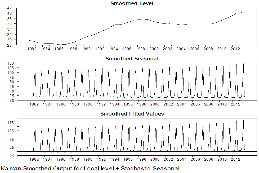 | Figure 9. Kalman Smoothed Output for local level with stochastic seasonal for Damaturu series |
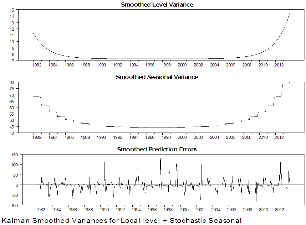 | Figure 10. Kalman Smoothed Output for local level with stochastic seasonal for Damaturu series |
In order to detect any systematic and haphazard structural breaks, we employed the cumulative sum (CUSUM) and cumulative sum squares (CUSUMSQ) introduced by Brown et al. (1975) to the residuals of the fitted model. The results of the CUSUM test are displayed in figure 11 and 12. Figure 11 indicates that there was a structural break around 1998 – 1999. Similarly, figure indicates the possibility of a structural break in the year 1990.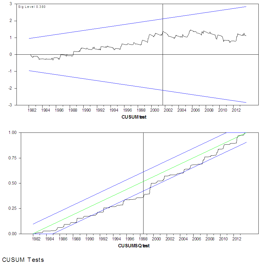 | Figure 11. The CUSUM and CUSUMSQ Structural Break test for Maiduguri Rainfall |
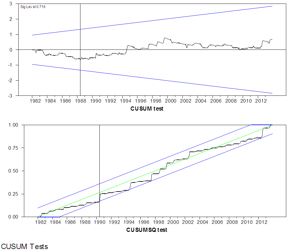 | Figure 12. The CUSUM and CUSUMSQ Structural Break test for Damaturu Rainfall |
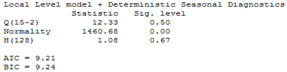
Table 5 indicates that the diagnostic tests for independence, homoscedasticity, and normality of the residuals for the fitted Maiduguri model are all satisfactory. These tests indicate that the residuals satisfy all of the assumptions of the models since the p-value associated with all the tests are insignificant at the conventional 0.05 significance level. Also, from table 6, the diagnostic tests for independence and homoscedasticity of the residuals are satisfactory for Damaturu fitted model, while that of normality is not satisfactory, which suggests that the residuals satisfy the two most important assumptions of the models as discussed in section 3. However, the residuals are higher at the beginning and end of the sample, as theoretically expected, since the smoothed states are calculated by a backwards recursions. Hence, the uncertainty in the estimation is higher at the beginning of the backward recursions, unlike the Kalman filtering that uses a forward recursion. We now present the results of analysis of Maiduguri and Damaturu rainfall time series with a local level model with a deterministic seasonal.Table 5. Diagnostics Results for Local Level Model with Stochastic Seasonal for Maiduguri Series
 |
| |
|
Table 6. Diagnostics Results for Local Level Model with Stochastic Seasonal for Damaturu Series
 |
| |
|
Table 7. Estimation Results for Local Level Model with Deterministic Seasonal for Maiduguri Rainfall Series (1981:1-2013:12)
 |
| |
|
The estimation results display above shows that the estimated hyperparameters (disturbance variances) of the measurement equation is significant while that of the level equation is not significant. Also, there are 396 observations in our series; however, the estimation is done using only the final 384 observations. This is because 12 diffuse initial state values are estimated (11 for the seasonal components and 1 for the local level components).We perform the Kalman filtering and smoothing based on these two estimates. We present the results of the Kalman filter estimates of the local level model with deterministic seasonal for Maiduguri and Damaturu in figure 13 to 16 and Kalman smoothed estimates of the local level model with deterministic seasonal in figure 16 and 19.Figures 13 and 16 present the output of the Kalman filtering of the local level model with deterministic seasonality for Maiduguri and Damaturu respectively. The output is very similar to the output of the local level model with stochastic seasonal (this is because the variance is small and insignificant), the evolution of Maiduguri and Damaturu rainfall is reflected by the estimated level component and is presented in the upper graph of figure 13 and 14. The plots also indicates that the period of highest level of rainfall in Maiduguri and Damaturu occurred in 2006 and 2000 respectively, while the lowest level occurred in 1986 and 1988-1989 respectively. Figure 14 also reveals that the Kalman filtered state variances converges to zero, while the filtered seasonal variance converges to a constant value. From figure 16, the filtered level variance converges to constant values as the sample size increases which empirically confirms that the local level model has a steady state solution.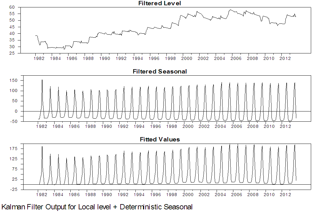 | Figure 13. Kalman Filter Output for local level with deterministic seasonal for Maiduguri series |
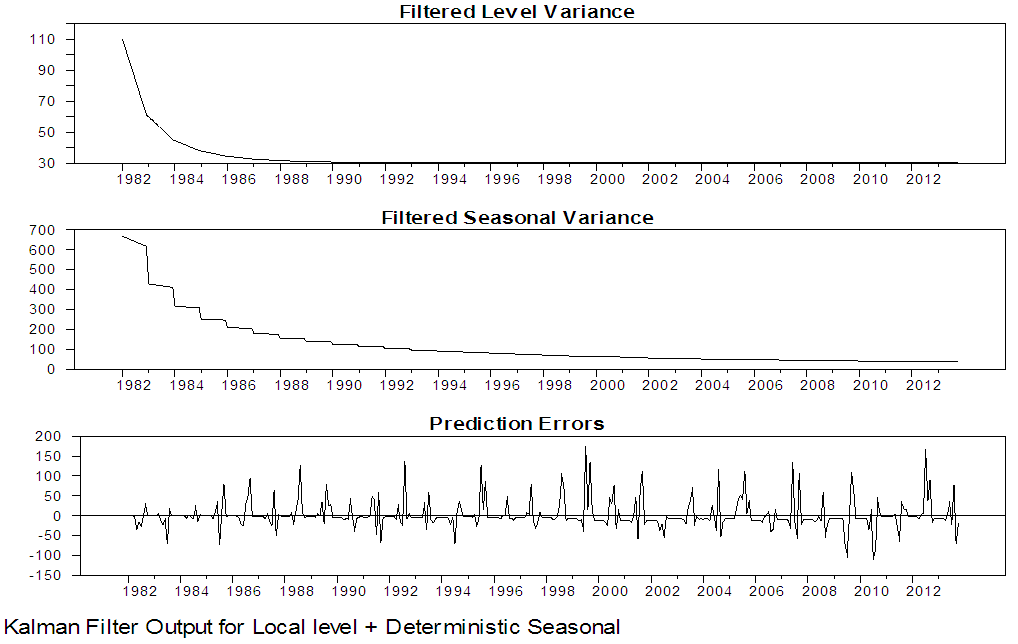 | Figure 14. Kalman Filter Output for local level with deterministic seasonal for Maiduguri series |
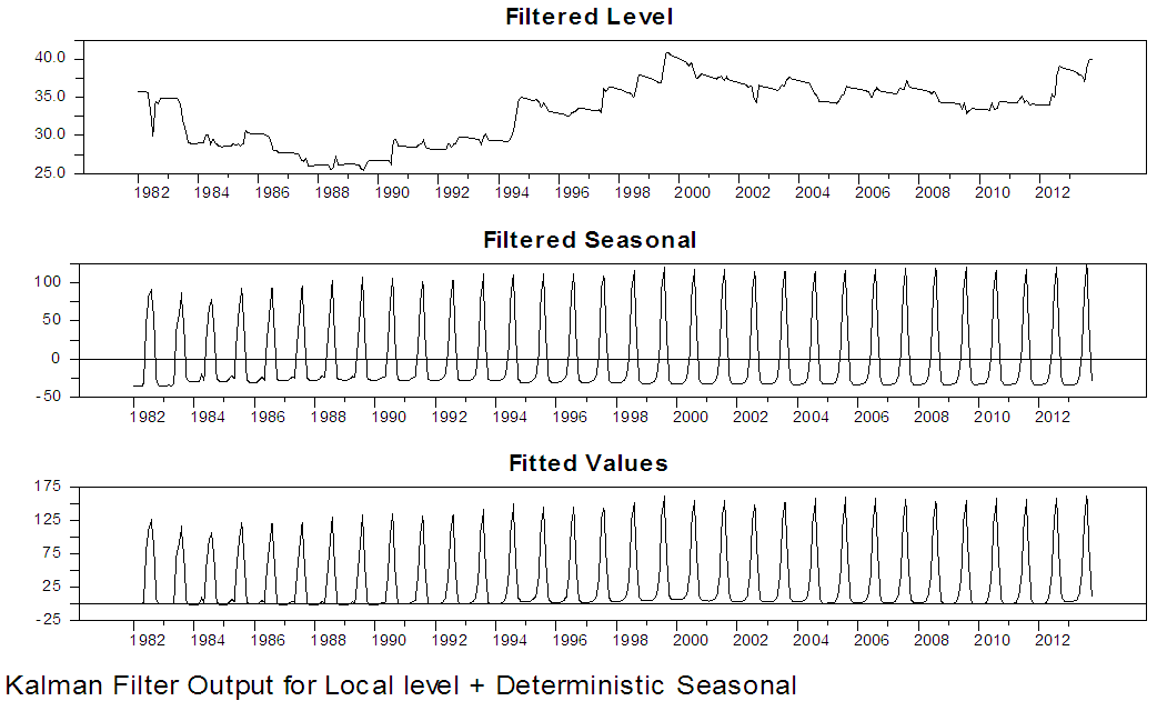 | Figure 15. Kalman Filter Output for local level with deterministic seasonal for Damaturu series |
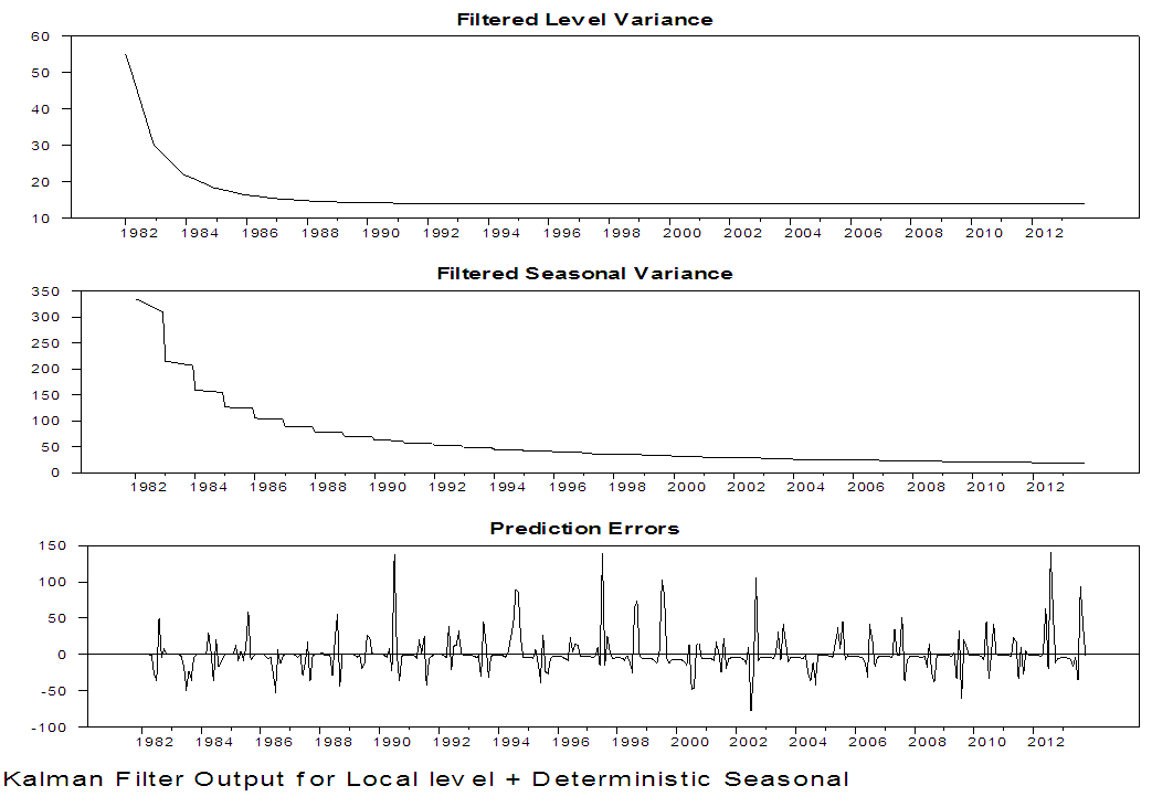 | Figure 16. Kalman Filter Output for local level with deterministic seasonal for Damaturu series |
Figures 17 to 20 present the output of the Kalman smoothing recursion estimates of the level, seasonal and the fitted values of the series together with the state variances of the level and seasonal component and the smoothed prediction errors for Maiduguri and Damaturu series. Comparing the graphs of the Kalman filtered level and the smoothed level in figure 13 and 15 and figure 17and 19, we see that the graph in figure 17 and 19 is smoother than that of figure 13 and15 for both states. However, the constant seasonal pattern in the series is clearly apparent in figure 18 and 20.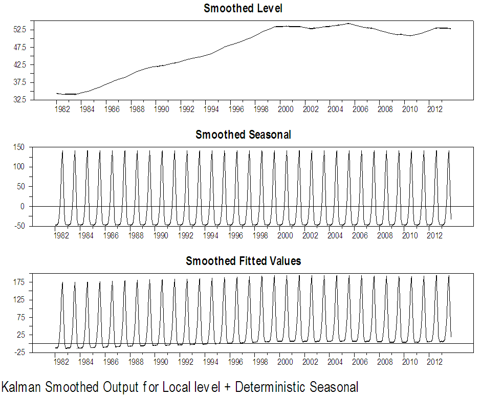 | Figure 17. Kalman Smoothed Output for local level with deterministic seasonal for Maiduguri series |
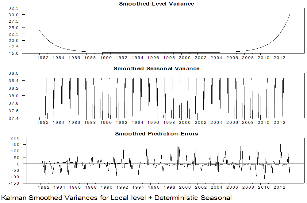 | Figure 18. Kalman Smoothed Output for local level with deterministic seasonal for Maiduguri series |
 | Figure 19. Kalman Smoothed Output for local level with deterministic seasonal for Damaturu series |
 | Figure 20. Kalman Smoothed Output for local level with deterministic seasonal for Damaturu series |
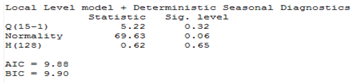
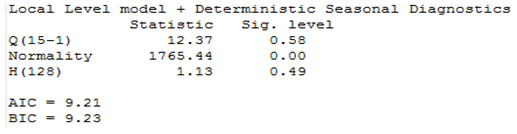
From table 8 and 10, the results of the diagnostic tests for the residuals of the local level model with deterministic seasonal are again satisfactory except for the normality of Damaturu. From table 9, the assumption of independence, homoscedasticity and normality are satisfied at the conventional level while table 10 indicates that the assumption of normality is not satisfied at conventional significance level.Table 8. Estimation Results for Local Level Model with Deterministic Seasonal for Damaturu Rainfall Series (1981:1-2013:12)
 |
| |
|
Table 9. Diagnostics Results for Local Level Model with Deterministic Seasonal for Maiduguri Rainfall Series
 |
| |
|
Table 10. Diagnostics Results for Local Level Model with Deterministic Seasonal for Damaturu Rainfall Series
 |
| |
|
From the two competing model that is; local level stochastic and local level deterministic model, the Akaike Information Criterion (AIC) and the Bayesian Information Criterion (SIC) of the two models are examined to obtain the parsimonious model. Using the information criteria approach, models that yield smaller values for the criterion are preferred, and regarded as best fitting model. From table 5 and 6, the AIC and BIC for the local level model with stochastic seasonal are 9.89, 9.21 and 9.92, 9.24, for Maiduguri and Damaturu respectively, while the AIC and BIC for the local level model with deterministic seasonal displayed in table 9 and 10 are 9.88, 9.21 and 9.90, 9.23 for Maiduguri and Damaturu respectively. Hence, the local level model with deterministic seasonal is slightly better than the model with stochastic seasonal component. In addition, the log-likelihood values of the two models for the two states are almost identical -1954.62, -1820.29 and -1954.36, -1821.65 for the local level model with stochastic seasonal and the local level model with deterministic seasonal respectively. Hence, the improved fit of the local level model with deterministic model can completely be attributed to its greater parsimony. Commandeur and Koopman (2007) pointed out that, in state space modelling, a small and insignificant state disturbance variance indicates that the corresponding state component may as well be treated as a deterministic effect, resulting in a more parsimonious model. Therefore, the local level model with deterministic seasonal is able to model the dynamic features in the Maiduguri and Damaturu rainfall time series.
5. Conclusions
The variability in elements of climate such as rainfall and temperature exposes the country to the negative impact of climate change such as erratic rainfall, rise in temperature, desertification, low agricultural yield, drying up of water bodies, and sea level rise. This paper analysed the seasonal pattern of rainfall in Maiduguri and Damaturu in the state space framework. We employ the local level model with deterministic and stochastic seasonal to modelling the monthly rainfall of the two states. The AIC and BIC of the two state space models suggest that the local level model with deterministic seasonal provide a better fit to the data than the model with stochastic seasonal. The detection of deterministic seasonal in the two states implies that the rainfall fall patterns have little variability or indication of climate change as regards its rainfall element. In addition, the CUSUM test indicates the presence of structural breaks in 1998 and 1990 for Maiduguri and Damaturu respectively. This implies that there was abrupt change in the rainfall level in 1998 for Maiduguri area and in 1990 for Damaturu area. We, therefore, recommend that seasonality should be explicitly included in the modelling of seasonal time series data as the pattern of seasonality could be useful for important decision making. These techniques can be adopted to the analysis of time series drawn from other domains. In addition, measures should be put in place to curb human-made activities that are detrimental to the climate since the region is highly vulnerable to the impacts of climate change. All computations performed in this study are done using the RATS econometric time series software.
Annexure I. Geographical Map of the Study Area
 | Annexure 1 |
References
| [1] | Ampaw, E. M. et al. (2013) Time Series Modelling of Rainfall in New Juaben Municipality of the Eastern Region of Ghana. International Journal of Business and Social Science. (4), p.116-129. |
| [2] | Brown, R.L., Durbin, J., & Evans, J.M. (1975). Techniques for testing the constancy of regression relationships over time. Journal of the Royal Statistical society, series B, 37, 149-192. |
| [3] | Dike, I.J. and Jibasen, D. (1997) Statistical Modelling Of Rainfall in Some Nigerian Cities. Unpublished article, p.38 – 43. |
| [4] | Dikko, H. G., David, I. J. and Bakari H.R.(2013) Modeling the Distribution of Rainfall Intensity using Quarterly Data. IOSR Journal of Mathematics. 9, p.11-16. |
| [5] | Durbin, J. and Koopman, S. (2001) Time Series Analysis by State Space Methods. United State: Oxford University Press. |
| [6] | Igwenagu, C. M (2015) Trend Analysis of Rainfall Pattern in Enugu State, Nigeria. European Journal of Statistics and Probability. 3 (3), p.12-18. |
| [7] | Jacques, J.F. and Koopman, S.J. (2007). An Introduction to State Space Analysis. United State: Oxford University Press. |
| [8] | Kim, C.J. and Nelson, C.R. (1999). State-Space Models with Regime Switching. Cambridge: MIT Press. |
| [9] | Koopman, S. and Durbin, J. (2014). Time Series Analysis by State Space Methods, 2nd Edition, United State: Oxford University Press. |
| [10] | Peter, M.W. (2000). Modelling Seasonality and Trends in Daily Rainfall Data. Unpublished article. p.985-991. |
| [11] | Ramana, R.V., Krishna, B. and Kumar, S.R. (2013) Monthly Rainfall Prediction Using Wavelet |
| [12] | Neural Network Analysis. Journal of Water Resources Management. 27, p.3697-3711. |
| [13] | Wee, P.MJ. and Shitan, M. (2013). Modelling Rainfall Duration And Severity Using Copula. SrinLankan Journal of Applied Statistics, 14-1, p.13 – 26. |
| [14] | West, M. and Harrison, J. (1997). Bayesian Forecasting and Dynamic Models, 2nd Edition. Springer-Verlag, New York. |
| [15] | Yusof, F.and Kane, I.L. (2012) Modelling Monthly Rainfall Time Series Using Ets State Space and Sarima Models. International Journal of Current Research. 4 (9), p. 195-200. |

 Abstract
 Reference
 Full-Text PDF
 Full-text HTML