1. Introduction

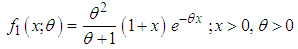
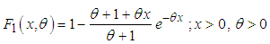
The important lifetime distributions for modeling lifetime data available in statistical literature are exponential, Lindley, Akash, Shanker, Aradhana, Sujatha, Amarendra, gamma, lognormal, and Weibull. The exponential, Lindley, Akash, Shanker, Aradhana, Sujatha, Amarendra and Weibull distributions are easy to apply for modeling lifetime data than the gamma and the lognormal distributions because the survival functions of the gamma and the lognormal distributions cannot be expressed in closed forms and both require numerical integration. Exponential, Lindley, Akash, Shanker, Aradhana, Sujatha and Amarendra distributions consists of one parameter and Lindley, Akash, Shanker, Aradhana, Sujatha and Amarendra distributions have advantage over exponential distribution that the exponential distribution has constant hazard rate whereas Lindley, Akash, Shanker, Aradhana, Sujatha and Amarendra distributions have monotonically increasing hazard rate. Further, the nature of Amarendra distribution is more flexible than exponential, Lindley, Akash, Shanker, Aradhana, and Sujatha distributions for modeling lifetime data.

The probability density function (p.d.f.) and the cumulative distribution function (c.d.f.) of Lindley (1958) distribution are given by

(1.1)

(1.2)

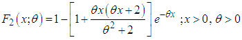
The density (1.1) is a two-component mixture of an exponential distribution and a gamma distribution with their mixing proportions and respectively. Ghitany et al (2008) have discussed various properties of this distribution and showed that in many ways (1.1) provides a better model for some applications than the exponential distribution. The Lindley distribution has been modified, extended, mixed and generalized suiting their applications in different fields of knowledge by many researchers including Sankaran (1970), Zakerzadeh and Dolati (2009), Nadarajah et al (2011), Deniz and Ojeda (2011), Bakouch et al (2012), Shanker and Mishra (2013 a, 2013 b, 2016), Shanker and Amanuel (2013), Shanker et al (2013), Elbatal et al (2013), Ghitany et al (2013), Merovci (2013), Ashour and Eltehiwy (2014), Oluyede and Yang (2014), Singh et al (2014), Sharma et al (2015), Shanker and Hagos (2015), Alkarni (2015), Pararai et al (2015), Abouammoh et al (2015), Shanker et al (2015, 2016 a, 2016 b, 2016 c) are some among others.

The probability density function (p.d.f.) and the cumulative distribution function (c.d.f.) of Akash distribution introduced by Shanker (2015 a) are given by

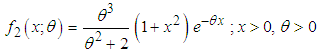(1.3)

(1.4)

The density (1.3) is a two-component mixture of an exponential distribution and a gamma distribution with their mixing proportions and respectively. Shanker (2015 a) has discussed its various mathematical and statistical properties including its shape, moment generating function, moments, skewness, kurtosis, hazard rate function, mean residual life function, stochastic orderings, mean deviations, distribution of order statistics, Bonferroni and Lorenz curves, Renyi entropy measure, stress-strength reliability, estimation of parameter and applications. Shanker et al (2016 c) has detailed and critical study about modeling and analyzing lifetime data from various fields of knowledge using one parameter Akash, Lindley and exponential distributions. Shanker (2016 a) has obtained Poisson mixture of Akash distribution named, Poisson-Akash distribution (PAD) and discussed its various mathematical and statistical properties, estimation of its parameter and applications for various count data-sets. Further, Shanker (2016 b, 2016 c) has also obtained the size-biased and zero-truncated versions of PAD, derived their important mathematical and statistical properties, and discussed the estimation of parameter and applications for count data-sets.

The probability density function (p.d.f.) and the cumulative distribution function (c.d.f.) of Shanker distribution introduced by Shanker (2015 b) are given by

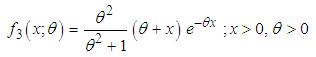(1.5)

(1.6)

The density (1.5) is a two-component mixture of an exponential distribution and a gamma distribution with their mixing proportions and respectively. Shanker (2015 b) has discussed its various mathematical and statistical properties including its shape, moment generating function, moments, skewness, kurtosis, hazard rate function, mean residual life function, stochastic orderings, mean deviations, distribution of order statistics, Bonferroni and Lorenz curves, Renyi entropy measure, stress-strength reliability, estimation of parameter and applications. Shanker (2016 d) has obtained Poisson mixture of Shanker distribution named Poisson-Shanker distribution (PSD) and discussed its various mathematical and statistical properties, estimation of its parameter and applications for various count data-sets. Shanker and Hagos (2016 a, 2016 b) have obtained the size-biased and zero-truncated versions of Poisson-Shanker distribution (PSD), derived their interesting mathematical and statistical properties, discussed the estimation of parameter and applications for count data-sets from different fields of knowledge.

The probability density function (p.d.f.) and the cumulative distribution function (c.d.f.) of Aradhana distribution introduced by Shanker (2016 e) are given by

(1.7)

(1.8)

The density (1.7) is a three-component mixture of an exponential distribution, a gamma distribution, and a gamma distribution with their mixing proportions , and , respectively. Shanker (2016 e) has discussed its various statistical and mathematical properties, estimation of parameter and applications for modeling lifetime data from biomedical science and engineering. Shanker (2016 f) has obtained Poisson-Aradhana distribution (PAD), a Poisson mixture of Aradhana distribution and showed that PAD gives a better fit than Poisson-distribution and Poisson-Lindley distribution (PLD) for modeling count data. Further, Shanker and Hagos (2016 c, 2016 d) have derived size-biased and zero-truncated versions of PAD and discussed their mathematical and statistical properties, estimation of parameter using maximum likelihood estimation and method of moments and discussed their applications.

The probability density function (p.d.f.) and the cumulative distribution function (c.d.f.) of Sujatha distribution introduced by Shanker (2016 g) are given by

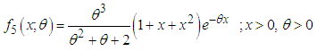(1.9)

(1.10)

The density (1.9) is a three-component mixture of an exponential distribution. a gamma distribution, and a gamma distribution with their mixing proportions , and respectively. Shanker (2016 g) has discussed its various mathematical and statistical properties including its shape, moment generating function, moments, skewness, kurtosis, hazard rate function, mean residual life function, stochastic orderings, mean deviations, Bonferroni and Lorenz curves, stress-strength reliability, some amongst others. Further, Shanker (2016 h) has obtained Poisson mixture of Sujatha distribution named Poisson-Sujatha distribution (PSD) and discussed its various mathematical and statistical properties, estimation of its parameter and applications for various count data-sets. Shanker and Hagos (2016 e, 2016 f) have obtained the size-biased and zero-truncated versions of Poisson-Sujatha distribution (PSD), derived their interesting mathematical and statistical properties, and discussed their estimation of parameter and applications for count data-sets. Shanker and Hagos (2016 g) has detailed study about applications of PSD for modeling count data from biological sciences. Shanker and Hagos (2016 h) has also done an extensive study on comparative study of zero-truncated Poisson, Poisson-Lindley and Poisson-Sujatha distribution and shown that in most of the data-sets from demography and biological sciences zero-truncated Poisson-Sujatha distribution gives much closer fit.

The probability density function and the cumulative distribution function of Amarendra distribution introduced by Shanker (2016 i) are given by

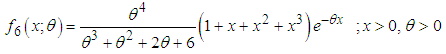(1.11)

(1.12)

Shanker (2016 i) has shown that the Amarendra distribution is a four component mixture of exponential distribution, a gamma distribution, a gamma distribution and a gamma distribution with their mixing proportions,, , and respectively. Shanker (2016 i) has done a detailed study of its various mathematical and statistical properties, estimation of its parameter and its applications. It has been observed that it provides a better model than exponential, Lindley and Sujatha distributions for modeling lifetime data. Shanker (2016 j) has also obtained a Poisson mixture of Amarendra distribution and named it ‘Poisson-Amarendra distribution’ and discussed its various properties, estimation of its parameter and its applications. Further, Shanker and Hagos (2016 i, 2016 j) have obtained size-biased and zero-truncated versions of Poisson-Amarendra distribution and discussed their properties, estimation of their parameter and its applications in different fields of knowledge.

The Probability density function (p.d.f.)of new one parameter lifetime distribution can be introduced as

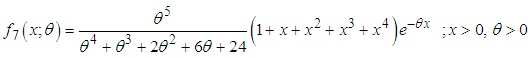(1.13)

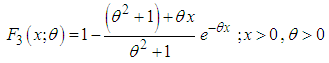
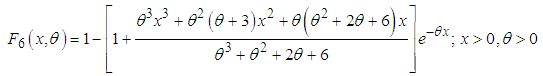
We would name this distribution as, ‘Devya distribution’. It can be easily shown that Devya distribution is a five component mixture of exponential distribution, a gamma distribution, a gamma distribution, a gamma distribution and a gamma distribution with their mixing proportions , , , , and respectively.

The corresponding cumulative distribution function (c.d.f) of Devya distribution (1.13) can be obtained as

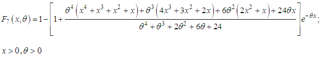(1.14)

The graphs of the p.d.f. and the c.d.f. of Devya distribution for different values of are shown in figures 1(a) and 1(b).

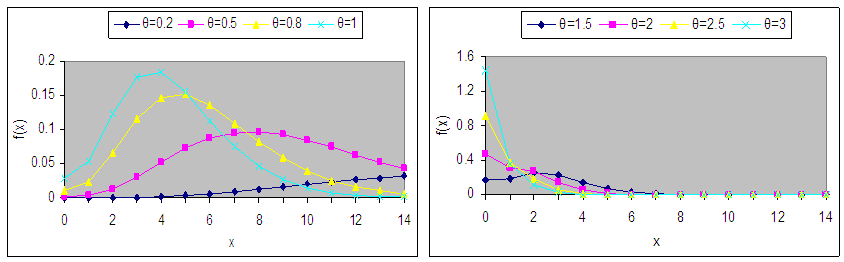Figure 1(a). Graphs of the p.d.f. of Devya distribution for selected values of the parameter θ

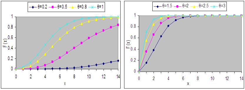Figure 1(b). Graphs of the c.d.f. of Devya distribution for selected values of the parameterθ

2. Moments and Related Measures

The moment generating function of Devya distribution (1.13) can be obtained as

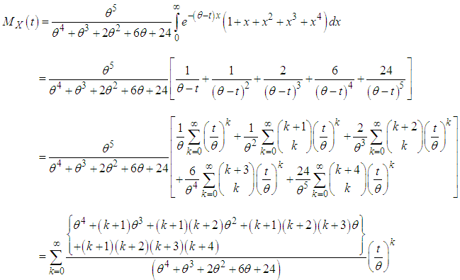The the moment about origin, of Devya distributon (1.13), obtained as the coefficient of in , can be given by

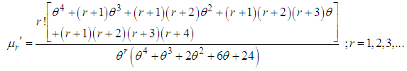Thus the first four moments about origin of Devya distribution (1.13) can be obtained as

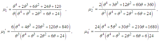Using the relationship between moments about mean and moments about origin, the moments about mean of Devya distribution (1.13) are obtained as

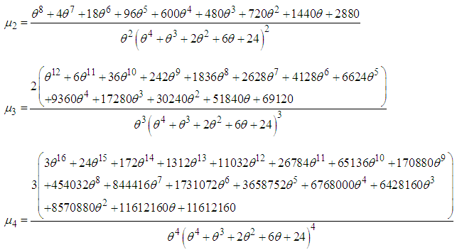The coefficient of variation, coefficient of skewness, coefficient of kurtosis and index of dispersion of Devya distribution (1.13) are thus obtained as

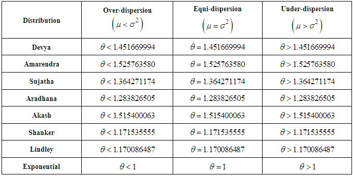
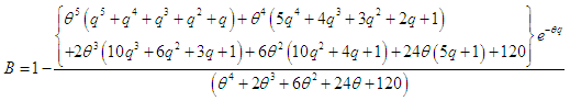
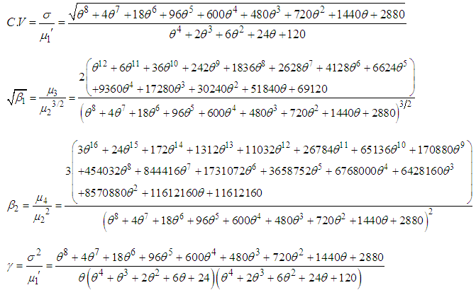The condition under which Devya distribution is over-dispersed, equi-dispersed, and under-dispersed has been given along with conditions under which Amarendra, Sujatha, Aradhana, Akash, Shanker, Lindley and exponential distributions are over-dispersed, equi-dispersed, and under-dispersed in table 1.

Table 1. Over-dispersion, equi-dispersion and under-dispersion of Devya, Amarendra, Sujatha, Aradhana, Akash, Shanker, Lindley and exponential distributions for varying values of their parameter θ

3. Hazard Rate Function and Mean Residual Life Function

Let be a continuous random variable with p.d.f. and c.d.f. . The hazard rate function (also known as the failure rate function) and the mean residual life function of are respectively defined as

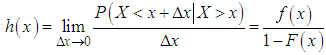(3.1)

(3.2)

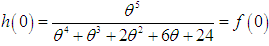
The corresponding hazard rate function, and the mean residual life function, of Devya distribution are thus given by

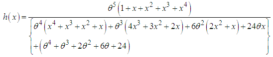(3.3)

and

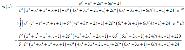(3.4)

It can be seen that and 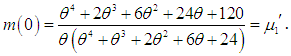. The graphs of and of Devya distribution (1.13) for different values of its parameter are shown in figures 3(a) and 3(b), respectively.

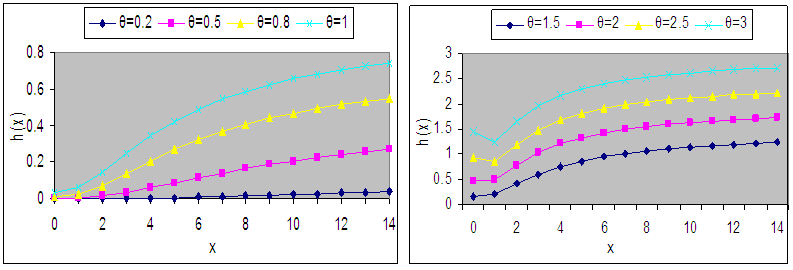Figure 2(a). Graphs of h(x) of Devya distribution for selected values of the parameter θ

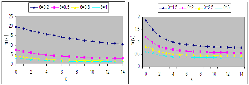Figure 2(b). Graphs of m(x) of Devya distribution for selected values of the parameter θ

It is also obvious from the graphs of and that is decreasing function of for and and is monotonically increasing function of other values of and , whereas is monotonically decreasing function of and .

4. Stochastic Orderings

Stochastic ordering of positive continuous random variables is an important tool for judging the comparative behaviour of continuous distributions. A random variable is said to be smaller than a random variable in the

(i) stochastic order if for all

(ii) hazard rate order if for all

(iii) mean residual life order if for all

(iv) likelihood ratio order if decreases in.

The following results due to Shaked and Shanthikumar (1994) are well known for establishing stochastic ordering of continuous distributions

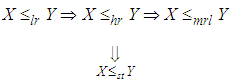The Devya distribution is ordered with respect to the strongest ‘likelihood ratio’ ordering as shown in the following theorem:

Theorem: Let Devya distributon and Devya distribution. If , then and hence , and .

Proof: We have

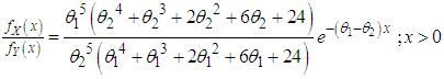Now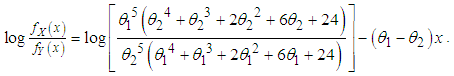

This gives

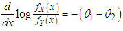Thus for 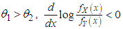. This means that and hence , and.

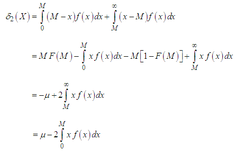
5. Mean Deviations

The amount of scatter in a population is evidently measured to some extent by the totality of deviations from the mean and the median. These are known as the mean deviation about the mean and the mean deviation about the median and are defined by

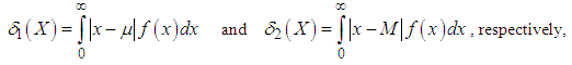where and .

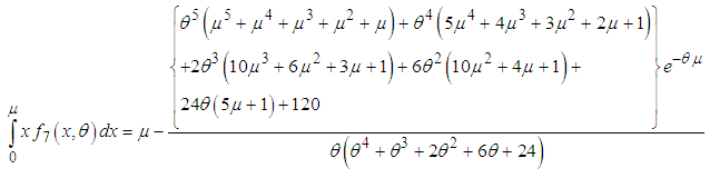
The expressions for and , can be calculated using the following relationships

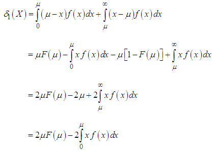(5.1)

and

(5.2)

Using p.d.f. (1.13) and the mean of Devya distribution, we get

(5.3)

(5.4)

Using expressions (5.1), (5.2), (5.3), and (5.4), the expressions for and of Devya distribution, after some algebraic simplification, are obtained as

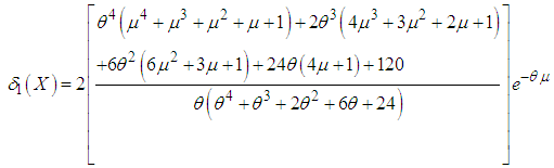(5.5)

and

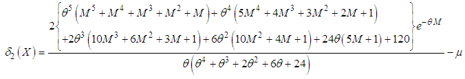(5.6)

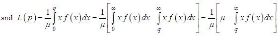
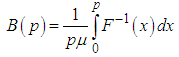
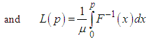
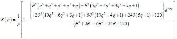
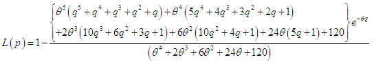
6. Bonferroni and Lorenz Curves

The Bonferroni and Lorenz curves (Bonferroni, 1930) and Bonferroni and Gini indices have applications not only in economics to study income and poverty, but also in other fields like reliability, demography, insurance and medicine. The Bonferroni and Lorenz curves are defined as

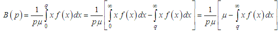(6.1)

(6.2)

respectively or equivalently

(6.3)

(6.4)

respectively, where and .

The Bonferroni and Gini indices are thus defined as

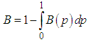(6.5)

(6.6)

respectively.

Using p.d.f. of Devya distribution (1.13), we get

(6.7)

Now using equation (6.7) in (6.1) and (6.2), we get

(6.8)

and

(6.9)

Now using equations (6.8) and (6.9) in (6.5) and (6.6), the Bonferroni and Gini indices of Devya distribution are obtained as

(6.10)

(6.11)

7. Estimation of Parameter

7.1. Maximum Likelihood Estimation

Let be a random sample of size from Devya distribution (1.13). The likelihood function, of Devya distribution is given by

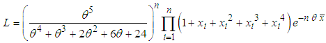and so the natural log likelihood function as

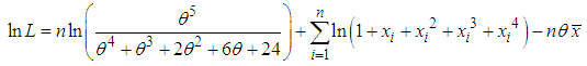where is the sample mean. Now

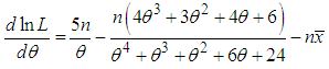The maximum likelihood estimate (MLE), of is the solution of the equation and is given by the solution of the following fifth degree polynomial equation

(7.1.1)

7.2. Method of Moment Estimation

Equating the population mean to the sample mean , the method of moment estimate (MOME) of of Devya distribution is found as the solution of the same fifth degree polynomial equation (7.1.1), confirming that the MLE and MOME of for Devya distribution are the same.

8. Goodness of Fit and Applications

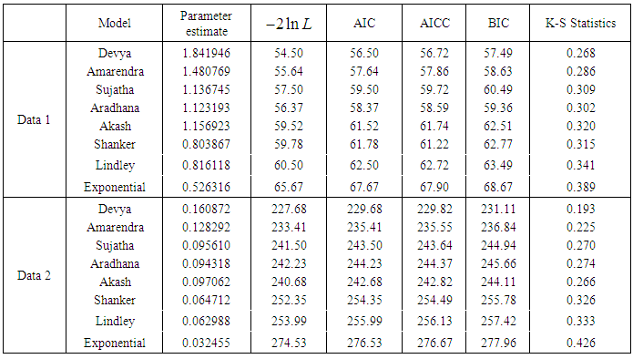
In this section, the goodness of fit and applications of Devya distribution to two real data sets using maximum likelihood estimate has been presented and the fit has been compared with one parameter exponential, Lindley, Shanker, Akash, Aradhana, Sujatha and Amarendra distributions. The following two real lifetime data-sets, first from medical science and the second from engineering has been considered.

Data set 1: The first data set represents the lifetime’s data relating to relief times (in minutes) of 20 patients receiving an analgesic and reported by Gross and Clark (1975, P. 105). The data are as follows:

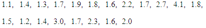Data set 2: The second data set is the strength data of glass of the aircraft window reported by Fuller et al (1994):

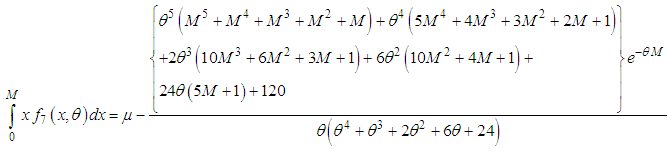
In order to compare the goodness of fit of these distributions, , AIC (Akaike Information Criterion), AICC (Akaike Information Criterion Corrected), BIC (Bayesian Information Criterion), and K-S Statistics ( Kolmogorov-Smirnov Statistics) for two real data sets have been computed and presented in table 2. The formulae for computing AIC, AICC, BIC, and K-S Statistics are as follows:

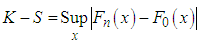, where k = the number of parameters, n = the sample size and is the empirical distribution function.

The best is the distribution which corresponds to the lower values of , AIC, AICC, BIC, and K-S statistics.

It is obvious from above table that Devya distribution gives much closer fit than exponential, Lindley, Shanker, Akash, Aradhana, Sujatha and Amarendra distributions and hence it may be preferred to exponential, Lindley, Shanker, Akash, Aradhana, Sujatha and Amarendra distributions for modeling various lifetime data.

Table 2. MLE’s, - 2lnL, AIC, AICC, BIC, and K-S Statistics of the fitted distributions of data sets 1 and 2

9. Concluding Remarks

A lifetime distribution named, ‘Devya distribution’ has been introduced to model lifetime data from biomedical science and engineering. Its moment generating function, moments about origin and moments about mean and expressions for skewness and kurtosis have been obtained. Other interesting properties of the distribution such as its hazard rate function, mean residual life function, stochastic ordering, mean deviations, Bonferroni and Lorenz curves, have been discussed. The estimation of its parameter has been discussed using maximum likelihood estimation and the method of moments. Two examples of real lifetime data - sets have been presented to show the goodness of fit of Devya distribution over one parameter exponential, Lindley, Shanker, Akash, Aradhana, Sujatha and Amarendra distributions.

NOTE: The paper is named in the name of Devya, a lovely grand child of my eldest brother Professor Shambhu Sharma, Department of Mathematics, Dayalbagh Educational institute, Dayalbagh, Agra, India.

ACKNOWLEDGEMENTS

The authors would like to thank the Editor-In-Chief and the referee for careful reading, constructive comments and suggestions which improved the quality of the paper.