M. Girish Babu
Department of Statistics, Government Arts and Science College, Meenchanda, Kozhikode, India
Correspondence to: M. Girish Babu, Department of Statistics, Government Arts and Science College, Meenchanda, Kozhikode, India.
| Email: |  |
Copyright © 2016 Scientific & Academic Publishing. All Rights Reserved.
This work is licensed under the Creative Commons Attribution International License (CC BY).
http://creativecommons.org/licenses/by/4.0/

Abstract
The Weibull and related models have been used in many applications for solving a variety of problems from many disciplines. Here we introduce a new family of distributions, namely Weibull-truncated negative binomial distribution (WTNB) and study some properties of it. Exponential-truncated negative binomial (ETNB) and Marshall-Olkin Weibull (MOW) distribution are special cases of this distribution. We have analyzed a real data set of serum creatinine values and found that this new distribution is a good fit to model the data, compared to Weibull, Gamma, Exponentiated Weibull, ETNB and MOW models.
Keywords:
Exponential – truncated negative binomial distribution, Marshall-Olkin family of distributions, Shannon entropy, Weibull distribution
Cite this paper: M. Girish Babu, On a Generalization of Weibull Distribution and Its Applications, International Journal of Statistics and Applications, Vol. 6 No. 3, 2016, pp. 168-176. doi: 10.5923/j.statistics.20160603.10.
1. Introduction
The Weibull distribution is a very popular distribution for modeling lifetime data and for modeling phenomenon with monotone failure rates. The distribution is named after Waloddi Weibull who was the first to promote the usefulness of this to model the breaking strength of materials (Weibull, 1939). A similar model was proposed earlier by Rosin and Rammler (1933) in the context of modeling the variability in the diameter of powder particles being greater than a specific size. The earlier known publication dealing with the Weibull distribution is a work by Fisher and Tippet (1928) where this distribution is obtained as the limiting distribution of the smallest extremes in a sample. Gumbel (1958) refers to the Weibull distribution as the third asymptotic distribution of the smallest extremes. The Weibull, and related models have been used in many applications, and for solving a variety of problems from many disciplines. Jayakumar and Girish (2015) studied some generalizations of Weibull distribution and related time series models.Marshall and Olkin (1997) proposed a new method of generating a family of distributions by introducing an additional parameter. Many authors have studied properties of various univariate distributions belonging to the family of Marshall-Olkin distributions, see, Alice and Jose (2003, 2005), Ghitany et al. (2005, 2007) and Jayakumar and Thomas (2008).A generalization of the Marshall-Olkin distributions was introduced by Nadarajah et al. (2013) as follows: Let  be a sequence of independent and identically distributed random variables with survival function
  . Le
. Le  be a truncated negative binomial random variable with parameters
  and
and  , that is,
 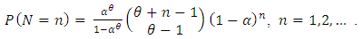 Consider
 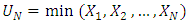 . Then
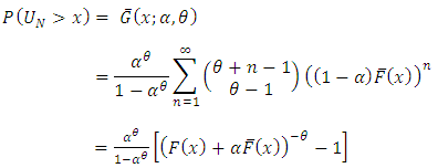 | (1.1) |
Similarly, if  and
and  is a truncated negative binomial random variable with parameters
  and
and  , then
  also has the survival function given in (1.1). Here note that in (1.1), if
  , then
  . If
. If  , then this family reduces to the family of Marshall – Olkin distributions. Thus the family of distributions described in (1.1) is a generalization of the family of Marshall-Olkin distributions.This family can be interpreted as follows. Suppose the failure times of a device are observed. Every time a failure occurs the device is repaired to resume function. Suppose also that the device is deemed no longer useable when a failure occurs that exceeds a certain level of severity. Let
  denote the failure times and
  denote the number of failures. Then
  will represent the time to the first failure of the device and
  will represent the life time of the device. Thus this family can be used to model both the time to the first failure and the life time.The probability density function of (1.1) is
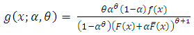 | (1.2) |
The hazard rate function is given by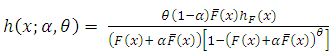 | (1.3) |
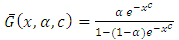
where  is the hazard rate corresponding to F.Nadarajah et al. (2013) introduced and studied a new family of distribution as exponential-truncated negative binomial distribution with parameters
  by substituting
  in the survival function (1.1).That is,
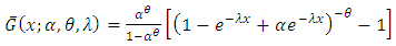 | (1.4) |
for  The paper is organized as follows. In section 2, we propose a new family of distributions, namely Weibull-truncated negative binomial distribution (WTNB). We study some properties of WTNB, such as the behavior of hazard rate, moments, Shannon and Renyi entropies and distributions of order statistics. Also the maximum likelihood method of estimation is used to obtain the estimates of parameters of WTNB. In section 3, we analyze a real data set of serum creatinine (mg.dL) values and found that WTNB is the most appropriate model for the data. The performance of the WTNB is compared to the well known models such as Weibull, Gamma, exponentiated Weibull, ETNB and Marshall-Olkin Weibull using AIC, BIC, K-S statistic and P-values.
2. Weibull-Truncated Negative Binomial Distribution
We propose a new family of distribution named as Weibull-truncated negative binomial (WTNB) distribution with parameters  and
and  by substituting
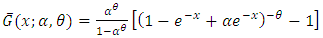
  in the survival function (1.1). Then,
 | (2.1) |
The probability density function of this distribution is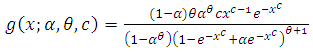 | (2.2) |
The hazard rate function is given by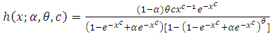 | (2.3) |
The shape of density and hazard rate functions are shown in the following figures.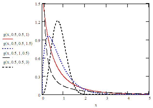 | Figure 2.1. Probability density function of WTNB distribution |
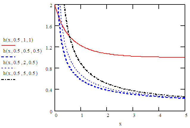 | Figure 2.2. Hazard rate function of WTNB distribution |
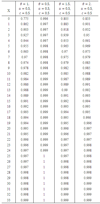
The cumulative probabilities at different choices of parameters are computed by using MATHCAD software and the results are shown in Table 2.1.Table 2.1. Cumulative Probabilities of WTNB distribution
 |
| |
|
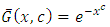
Some distributions arise as special cases of the 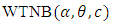 Case I : For
  ,
, | (2.4) |
This is the survival function of two parameter Exponential-truncated negative binomial distribution.Case II: For  ,
, | (2.5) |
This is the survival function of Marshall-Olkin extended Weibull distribution with parameters  .Case III: For
 | (2.6) |
This is the survival function of one parameter Weibull distribution.Case IV: For 
 | (2.7) |
This is the survival function of the generalized half logistic distribution.Case V: When  reduces to the one parameter Weibull distribution.A random sample from
  distribution can be simulated as
 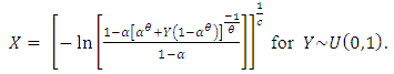 | (2.8) |
2.1. Moments
Suppose that X has the  distribution. The nth moment can be written as
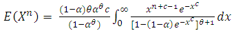 | (2.9) |
Taking  , (2.9) reduces to
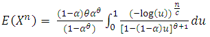 | (2.10) |
If  , then by the series expansion
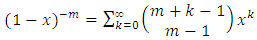 , equation (2.10) can be written as
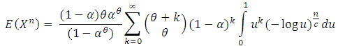 where
where 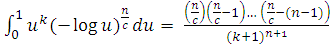 Therefore,
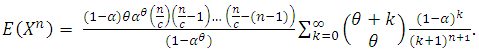 | (2.11) |
If  , then we have
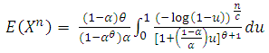 | (2.12) |
Taking  in equation (2.12) and using equation (2.6.5.3) of Prudnikov et al. (1986), we have
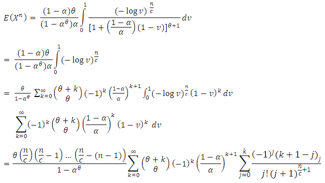 | (2.13) |
2.2. Shannon Entropy
Entropy is a measure of variation or uncertainty. The Renyi entropy of a random variable with probability density function  is defined as
 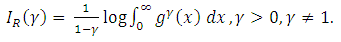 | (2.14) |
The Renyi entropy of 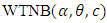 is
is 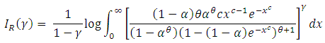 Letting
  , we have
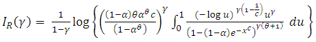 | (2.15) |
The Shannon entropy is given by | (2.16) |
2.3. Order Statistics
Let  are independent random variables having the
  distribution. Let
  denote the ith order statistic. The probability density function of
  is
is 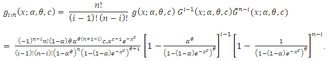 | (2.17) |
Using the binomial series expansion, the probability density function can be written as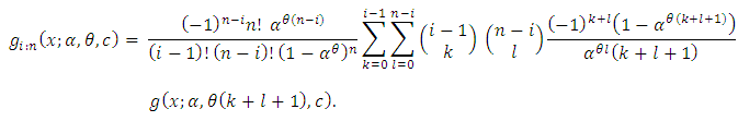 | (2.18) |
This shows that  is a finite mixture of WTNB random variables.
2.4. Estimation
For a given sample  , the log-likelihood function is given by
 | (2.19) |
The partial derivatives of the log-likelihood function with respect to the parameters are | (2.20) |
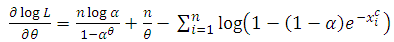 | (2.21) |
 | (2.22) |
Equating these partial derivatives equal to zero and solving these equations numerically, we get the maximum likelihood estimates of  .
.
3. Application
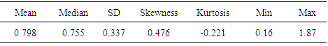
In this section, we analyze a real data set and found that WTNB distribution gives the best fit for the data. We consider a real data set of serum creatinine (mg/dL) value of 300 samples reported on February 2nd, 2016 at the Biochemistry Laboratory of Govt. Medical College, Calicut, Kerala. The data are follows:0.83 1.05 1.37 1.11 0.26 0.39 0.30 0.66 0.65 0.74 0.71 0.64 1.06 0.38 0.88 0.82 0.68 1.51 0.68 1.33 1.05 0.53 1.15 0.77 0.86 1.03 1.21 1.22 1.69 1.70 1.02 0.17 0.79 0.34 0.40 0.60 0.69 0.63 0.76 0.49 0.55 1.42 0.62 0.42 0.50 0.72 0.43 0.46 0.88 1.35 0.48 1.43 0.57 0.58 0.39 0.99 0.85 1.00 0.85 0.73 0.66 0.81 0.43 0.47 0.24 0.46 0.27 1.32 0.42 1.13 0.51 0.59 0.72 1.29 0.58 0.35 0.80 0.93 1.13 0.90 0.67 0.98 0.73 0.35 0.89 1.12 1.35 0.94 0.33 0.59 0.43 1.29 1.14 0.77 0.68 0.38 0.73 0.48 0.33 1.03 0.68 0.47 0.61 0.84 1.00 0.71 1.15 0.58 0.70 0.28 0.23 0.85 0.96 1.02 0.36 0.73 0.53 0.75 0.71 0.62 0.71 0.69 1.25 1.09 0.44 0.86 0.67 0.81 1.30 0.60 0.56 1.02 0.53 0.27 1.64 0.64 0.47 1.29 0.57 0.94 0.36 1.16 1.12 1.07 0.75 1.13 1.34 0.43 1.09 0.79 1.58 0.56 0.83 0.99 1.05 1.04 0.57 1.22 0.52 1.25 0.57 0.75 1.03 0.58 1.87 0.65 1.50 0.57 0.16 1.27 0.81 0.64 1.33 0.94 1.44 0.83 1.02 0.82 1.27 0.83 1.07 0.78 0.41 0.66 1.08 0.21 0.33 0.54 0.55 0.67 1.16 0.93 0.81 0.49 0.68 0.49 0.79 1.26 0.58 0.43 0.88 0.51 1.58 0.71 1.04 0.91 0.73 0.89 0.57 1.04 0.65 0.31 0.72 0.92 0.72 0.53 0.92 0.54 1.08 1.20 0.37 0.88 1.33 0.56 1.15 0.71 0.39 0.87 0.17 0.68 0.77 0.66 0.47 0.51 0.41 0.38 0.73 0.26 0.82 0.84 0.85 0.40 1.05 0.35 0.69 0.71 1.14 0.79 0.94 0.53 0.34 1.19 1.25 0.26 0.79 0.96 0.43 0.46 0.52 0.84 0.19 0.64 0.96 0.97 0.72 1.62 1.12 1.11 0.77 0.79 0.63 0.49 1.04 1.42 0.79 0.78 0.75 0.97 0.72 1.02 0.45 0.56 1.30 0.50 0.56 1.14 0.94 1.37 1.39 1.07 1.02 0.99 0.76 1.43 0.33 1.32 0.78 1.44 0.51 0.77 Creatine is a chemical made by the body and is used to supply energy mainly to muscle. Serum creatinine is a chemical waste product of creatine. Creatinine is removed from the body entirely by the kidneys. If kidney function is not normal, the creatinine level will increase. The normal range of creatinine is about 0.7 to 1.3 mg/dL.The descriptive measures of the 300 samples are as follows:Initially a histogram of the data is plotted and a normal curve is embedded in it and we observe that normal distribution is not suitable to model the data since the data is highly positively skewed.Table 3.1. Descriptive statistics of Creatinine (mg/dL)
 |
| |
|
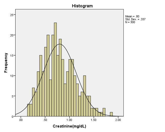 | Figure 3.1. Empirical structure of the serum creatinine data |
The P-P plot and Q-Q plot of the creatinine data is as follows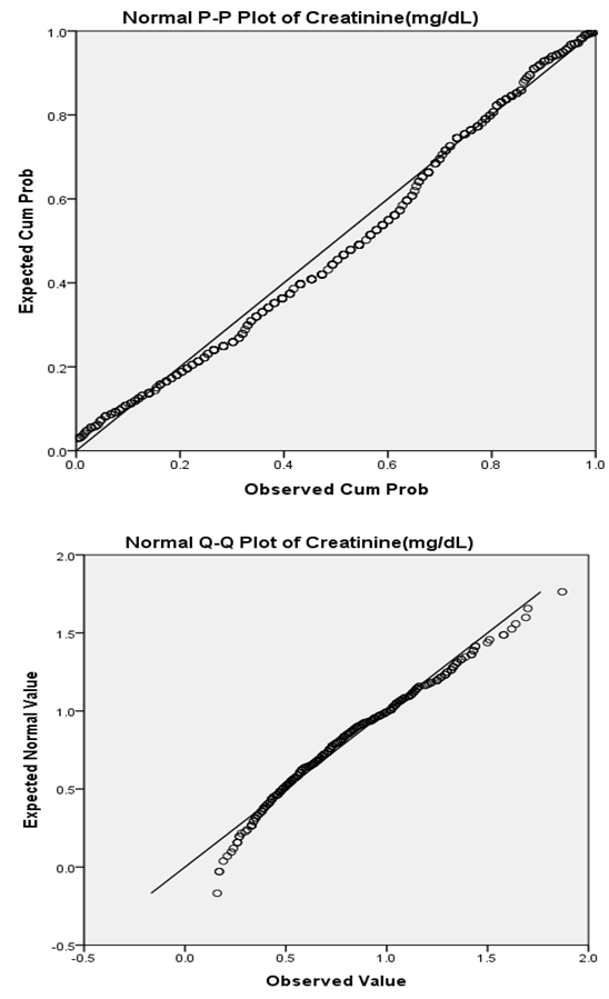 | Figure 3.2. P-P plot and Q-Q plot of the serum creatinine data |
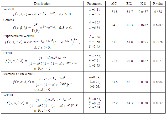
Since the data shows a positively skewed nature, the symmetrical distributions will not be a suitable choice. So we fitted the data using WTNB with three parameters and compared with the well known distributions like Weibull, Gamma, Exponentiated Weibull, Marshall-Olkin Weibull and ETNB. For comparing the goodness of fit of the model we used the information criteria, Akaike Information Criterion (AIC = -2 log L+2k), Bayesian Information Criterion (BIC = -2log L+k log n) and the Kolmogorov-Smirnov statistic, where k is the number of unknown parameters, log L is the log-likelihood function value and n is the sample size. The results are presented in Table 3.2.Table 3.2. Parameter estimates and goodness of fit statistics for various models fitted to the serum creatinine data
 |
| |
|
From the above Table 3.2., we can see that the WTNB distribution is the suitable model for the given data. The probability plots for the fitted models are presented in figure 3.3.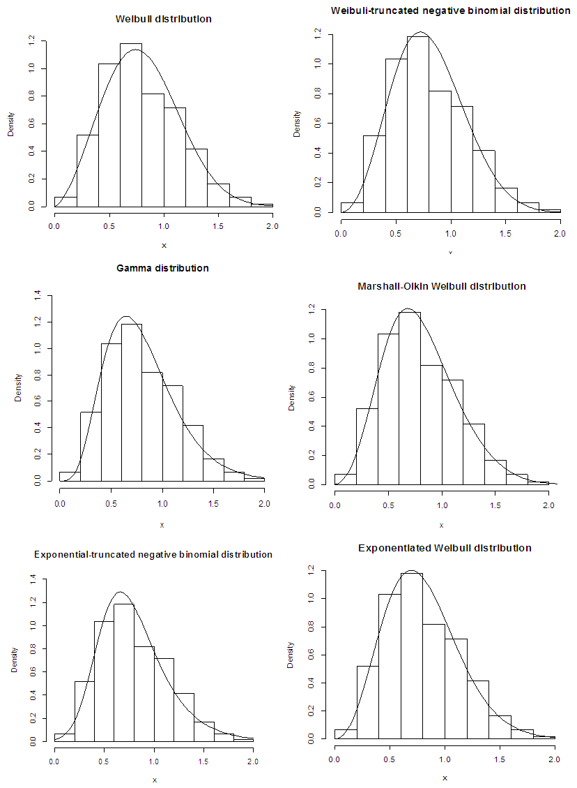 | Figure 3.3. Fitted probability density function for the serum creatinine (mg/dL) data |
We have used the nlm function of R software to compare the empirical distribution and the theoretical distribution of all the six distributions mentioned above. From the results out of the six fitted models, WTNB is closer to the empirical distribution of the serum creatinine data. The following figure shows the closeness of the distribution functions. 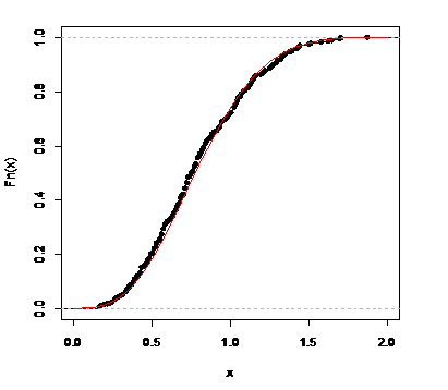 | Figure 3.4. WTNB distribution function and empirical distribution |
4. Conclusions
In the present paper, we have studied a new family of distributions, namely Weibull truncated negative binomial distributions. Some properties of this distribution such as hazard rate, moments, Shannon and Renyi entropies, distributions of order statistics are studied. This distribution is found to be the most appropriate model to fit the serum creatinine data compared to the Weibull, Gamma, Exponentiated Weibull, ETNB and MOW models. We hope that the new family will attract wider application in life time modeling.
References
| [1] | Alice, T. and K.K. Jose (2003): Marshall-Olkin Pareto process, Far East Journal of Theoretical Statistics, 9, 117-132. |
| [2] | Alice, T. and Jose, K.K. (2005): Marshall-Olkin semi-Weibull minification processes, Recent Advances in Statistical Theory and Applications, 1, 6-17. |
| [3] | Fisher, R.A. and Tippett, L.H.C. (1928): Limiting forms of the frequency distribution of the largest and smallest member of a sample, Proceedings of the Cambridge Philosophical Society, 24, 180-190. |
| [4] | Ghitany, M.E., Al-Hussaini, E.K. and Al-Jaralla, R.A. (2005): Marshall-Olkin extended Weibull distribution and its application to censored data, Journal of Applied Statistics, 32, 1025-1034. |
| [5] | Ghitany, M.E., Al-Awadgi, F.A. and Alkhalfan, I.A. (2007): Marshall-Olkin extended Lomax distribution and its application to censored data, Communication in Statistical Theory and Methods, 36, 1855-1866. |
| [6] | Gumbel, E.J. (1958): Statistics of Extremes, Columbia University Press, New York. |
| [7] | Jayakumar, K. and Girish, B.M. (2015): Some generalizations of Weibull distribution and related processes, Journal of Statistical Theory and Applications, 14, 425-434. |
| [8] | Jayakumar, K. and Thomas, M. (2008): On a generalization to Marshall-Olkin scheme and its application to Burr type XII distribution, Statistical Papers, 49, 421-439. |
| [9] | Marshall, A.W. and Olkin, I. (1997): A new method for adding parameter to a family of distributions with application to exponential and Weibull families, Biometrika, 84, 641-652. |
| [10] | Nadarajah, S., Jayakumar, K. and Ristic, M.M. (2013): A new family of lifetime models, Journal of Statistical Computation and Simulation, 83, 1389-1404. |
| [11] | Prudnikov, A.P., Brychkov, Y.A., and Marichev, O.I. (1986): Integrals and Series Vol.1, Gordon and Breach Sciences, Amsterdam, Netherlands. |
| [12] | Rosin, P. and Rammler, E. (1933): The laws governing the fineness of powdered coal, Journal of the Institute of Fuels, 6, 29-36. |
| [13] | Weibull, W. (1939): A statistical theory of the strength of material, Ingeniors Vetenskaps Akademiens Handligar Report No.151, Stockholm. |

 Abstract
 Reference
 Full-Text PDF
 Full-text HTML