-
Paper Information
- Next Paper
- Previous Paper
- Paper Submission
-
Journal Information
- About This Journal
- Editorial Board
- Current Issue
- Archive
- Author Guidelines
- Contact Us
International Journal of Statistics and Applications
p-ISSN: 2168-5193 e-ISSN: 2168-5215
2016; 6(3): 123-137
doi:10.5923/j.statistics.20160603.05

Statistical Models for Count Data with Applications to Road Accidents in Ghana
 Abstract
 Reference
 Full-Text PDF
 Full-text HTML
A. Y. Omari-Sasu , Adjei Mensah Isaac , R. K. Boadi
Department of Mathematics, Kwame Nkrumah University of Science and Technology, Kumasi, Ghana
Correspondence to: Adjei Mensah Isaac , Department of Mathematics, Kwame Nkrumah University of Science and Technology, Kumasi, Ghana.
| Email: |  |
Copyright © 2016 Scientific & Academic Publishing. All Rights Reserved.
This work is licensed under the Creative Commons Attribution International License (CC BY).
http://creativecommons.org/licenses/by/4.0/

Road accidents in Ghana seems to be on ascendency and the root causes have been attributed to issues such as human errors and superstitions. Since the occurrences of these accidents are discrete, they are often modelled using count regression models. It is therefore the purpose of this study to determine an appropriate count regression model that adequately fits road accidents in Ghana and determine the key predictors using the appropriate model with respect to the expected number of persons killed in road accidents. Several models were compared to fit count data that encounter the field of transportation. These models include Poisson, Negative Binomial (NB) and Conway-Maxwell-Poisson (CMP) models. In order to compare the performance of these models, the various model selection methods such as Deviance goodness of fit test, Akaike’s Information Criterion (AIC) and Bayesian Information Criterion (BIC) were employed. Because the values of Deviance goodness of fit test, AIC and BIC for the NB model was the smallest as compared to that of the Poisson and CMP models, it appeared that, the NB model performed best than the Poisson and CMP models. Base on the appropriate model selected (NB model), the key predictors that contributed significantly and also had a high effect on the expected or mean number of persons killed in road accidents within a particular period were Head-on collision as Collision type, Improper overtaking and Loss of control as Driver errors, Bus/Minibus as Type of vehicle, Fog/Midst as Weather condition and Night with street lights off as Light condition.
Keywords: AIC, BIC, Goodness of fit, Poisson model, Negative binomial model, CMP model, Count Data
Cite this paper: A. Y. Omari-Sasu , Adjei Mensah Isaac , R. K. Boadi , Statistical Models for Count Data with Applications to Road Accidents in Ghana, International Journal of Statistics and Applications, Vol. 6 No. 3, 2016, pp. 123-137. doi: 10.5923/j.statistics.20160603.05.
Article Outline
1. Introduction
- Road accident is defined as any activity that distracts the normal trajectory of moving vehicles in a manner that causes instability in the free flow of the vehicle. Road accidents in Ghana has been a serious concern to many Ghanaians in recent times. As a result of the tremendous effect of road accidents on human lives, properties and the environment as a whole, numerous researchers have come out with the causes, effects and recommendations to road accidents. These causes include drunk driving, over speeding and machine failure (Sagberg, Fosser and Saetermo (1997), Adams (1982) and National Road Safety Commission (2009)). Despite all these being done, yet every year the Ghana Statistical Service, Road Safety Commission and other organizations would report there is an increase in road accidents in the country (Annual Report, National Road Safety Commission. 2009).Researchers in recent times have been modelling road accidents with crash prevention models in various parts of the world. However, it is extremely tedious to just apply models which have worked in other area to data obtained from different countries due to the variations in the various factors pertaining in different countries (Fletcher et al., 2006). There has not been much statistical research work conducted with respect to accidents on urban roads in Ghana and this might have been as a result of inadequate information available on accidents on urban roads and its impact on human lives and the environment as a whole in the country.Salifu (2004) developed a forecasting model for traffic crashes for urban junctions with no road signs, Afukaar and Debrah (2007) on the other hand modelled traffic crashes for signalized urban junctions in Ghana and Akaah (2011) additionally modelled traffic crashes on rural highways in Ashanti region. Road accidents have always been attributed to human errors such as high alcoholic content in blood stream of some drivers, over speeding, wrong-overtaking among others. It has also been linked to poor road networks, poor surfacing of roads, witchcraft and death dying nature of some vehicles which ply the roads. It is however surprising that in spite of the numerous factors identified by researchers as causes of road accidents in Ghana and its consequences on human lives and properties; nobody has modelled the causes of accidents on urban roads and their contributions to the death of casualties in Ghana to authenticate the contributions of each of these factors to the casualties. It is therefore in light of this that this research is conducted in order to determine the appropriate count regression model that fits accident data with respect to the expected number of persons who will be killed via road accidents on urban roads in Ghana and additionally use the appropriate count regression model to investigate the key predictors of accidents that results in the death of casualties.
2. Related Works
- Numerous road accident models have been developed to estimate the expected number of accident frequencies on roads as well as to identify the various factors associated with the occurrence of accidents. It is not possible for regression models to account for each and every factor that affects accident occurrences (Persaud and Dzibik, 1993). Previous researchers have focused on the no-behavioural factors such as traffic flow characteristics, road geometry and environmental conditions. Persaud and Dzibik (1993), as the first accident modellers who worked on multilane road, investigated the relationship between freeway crash data and accident volumes. By using the hourly traffic, the model indicated that, a higher accident risk is associated with congestion and afternoon rush hour. Shankar et al., (1995) modelled the monthly accident frequency of rural motorway as a function of geometrics, weather conditions and their interaction and found it dangerous for the areas with large rainfall and snowfall to have steep grades and tight horizontal curves.Abdel and Radwan (2000) attempted to use Poisson regression model and then rejected it with the reason that, different mean and variance value of the dependent variable showed over-dispersion in the accident data. Consequently, the Negative binomial model also called the Poisson-Gamma mixture model was then adopted as a superior alternative model to accommodate the vehicle accident analysis for rural highways, arterial roadways, urban roads and rural motorways (Shankar et al., 1995; Lord, 2005; Montella, 2008; Pemmanaboina, 2005). Recently, a number of approaches have been proposed in the domain of accident models seeking improvement from traditional methods earlier discussed. For instance, El-Basyouny and Sayed (2006) proposed a modified Negative binomial regression technique which improved goodness of fit. Caliendo et al, (2007) on the other hand applied Negative Multinomial distribution to model multiple observations in the same road section at different years that may not be mutually independent. The generalized estimating equation was also used by researchers such as Abdel and Abdalla (2004) and Lord and Persaud (2000).In New Zealand, the generalized linear models (GLMs) have been used in accident research of different intersection types as a well as for two-lane roads. The earlier work usually emphasized on the effect of traffic volume. So far the effort to model accident likelihood on motorway in New Zealand have been minimized except the flow-only models presented by Turner (2011) and the Economic Evaluation Manual (2010).In order to obtain a valid and very accurate model that can fit accident data comparison and prediction, other researchers upon identifying the flaws in previous models tried different means by including more factors in the accident data analysis. Livneh and Hakkert (1972) researched into road accidents in Israel using employment and population data. On the other hand Susan and Partyka (1984) also modelled road accidents with the help of employment and population data. Research conducted by Andreassen (1985) raised serious objection to the use of death per vehicles licensed in order to make international comparison of road accident fatalities with the reason that it was found out that the two parameters were not linearly related overtime. As a result, he came out with a general formula;
 | (1) |
3. Method
- This research work mainly utilized secondary data obtained from the Building and Road Research Institute (BRRI) of the Council of Scientific and Industrial Research (CSIR). The data for the research was originally collected with the help of the Police accident report by the Motor Traffic and Transport Unit (MTTU) of the Ghana Police Service. This research work considered a data for five (5) years period from 2009 to 2013. The mean or expected number of persons killed in individual road accidents for the five years period was used as the dependent or response variable and other categorical variables such as collision type, weather conditions, light condition, type of vehicle and driver error as, the explanatory or independent variables.
3.1. Regression Models
- Count data, such as accident fatalities are better modelled using Poisson, Negative Binomial and Conway- Maxwell- Poisson regression models. Regardless of whether the assumed model is Poisson, Negative Binomial or Conway- Maxwell-Poisson, it will be assumed that the occurrences will be independent of each other. The three (3) types of count regression models are briefly explained as follows:
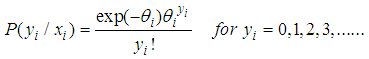
3.1.1. Poisson Regression
- The most basic model for event counts is the Poisson regression model. If the variance of the counts approximately equals the mean counts, then the Poisson regression model is expressed as:
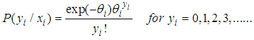 | (2) |
 is the number of counts (persons killed in accidents) for a particular period of time
 is the expected or mean number of counts (persons killed in road accidents) per period, which can be modelled as;
 | (3) |
 is the vector of the explanatory or independent variables and
  is the vector of unknown regression parameters. Equation 3 above as a result gives the indication that a unit increase in an
  increases
  by a multiplicative factor of
  . The main constraint of the Poisson regression model is that, the mean and the variance are approximately equal, that is;
 | (4) |
 | (5) |
 | (6) |
 must be set to zero as;
 | (7) |
3.1.2. Negative Binomial Model
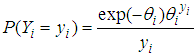
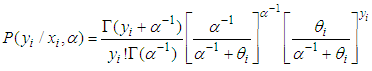
- The Negative Binomial model can be obtained from the mixture of Poisson and Gamma distributions and is expressed as;
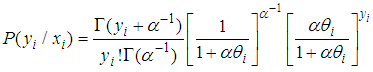 | (8) |
 is the number of road accidents for a road segment
  and
and  is the mean or expected number of persons killed in a road accidents per period, which can be expressed as;
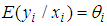
 The conditional mean and variance of the Negative Binomial distribution are
  and
and  respectively. Hence the NB model is over-dispersed and allows extra variation relative to the traditional Poisson model. It has more desirable properties than the Poisson model (Chin and Quddus, 2003). The variance of the Negative Binomial is significantly greater than the mean. The NB model,
  represents the dispersion parameter which allows or indicates the degree of over-dispersion. For instance, if
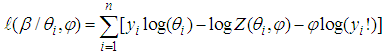
  the NB model reduces to the traditional Poisson model.The Log-likelihood function of the NB model is obtained from the following equation;
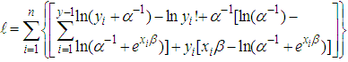 | (9) |
 and
and  as in the Poisson model, the iteration procedure or method of Newton Raphson is applied (Lee and Mannering, 2002).
3.1.3. Conway-Maxwell-Poisson Model
- The Conway-Maxwell-Poisson model (CMP) is a discrete probability distribution that generalizes the Poisson distribution by adding a parameter to model over-dispersion and also a member of the exponential family. The Conway-Maxwell-Poisson has a probability mass function of the form:
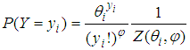 | (10) |
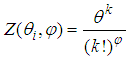 For
For  and
and . The function
  is an infinite series that converges for
  and
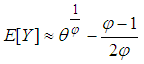
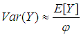
and .The CMP distribution shows that, there is a non-linear relationship between the ration of successive probabilities as displayed by;
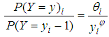 | (11) |
 | (12) |
 | (13) |
 | (14) |
 | (15) |
3.1.4. Conway-Maxwell-Poisson Generalized Linear Model
- The Conway-Maxwell-Poisson distribution was extended into the Classical General Linear Model framework by Sellers and Schumeli (2008). Hence the CMP distribution is a member of the linear exponential family as displayed by;
 | (16) |
 | (17) |
3.2. Selecting Over-Dispersed Models
- In order to test whether the data is over-dispersed or not, we test the following hypothesis;
 where
where  is a dispersion parameter.The corresponding test statistic is;
 | (18) |
 and for large sample size, the z has an approximate standard normal distribution. We therefore reject
  at alpha level of significance if
  If we reject the null hypothesis as a result then it gives an indication that the data is over-dispersed hence the Negative Binomial and the CMP models will be more appropriate compared to the Poisson model.
3.3. Model Specification
- Models considered in this research work has the mean or expected number of persons killed in road accidents within a particular period of time as a function of the categorical variable; collision type, driver error, type of vehicle, weather condition and light condition. Each model parameterizes;
 | (19) |
 individuals, CT denotes the Collision Type, DE represents the Driver Errors, TV is the Type of Vehicle, LC as the Light Condition and WC representing the Weather Condition.
3.4. Parameter Estimation
- The Maximum Likelihood Estimation (MLE) method has been considered due to the fact that all the models involved in the research work can be estimated using the MLE procedure. To evaluate the models involved in the research work, it is necessary to examine the significance of the variables included in the model. For a better model, the estimated regression coefficients have to be statistically significant.
3.5. Model Selection Methods
3.5.1. Goodness of Fit
- After fitting the various models involve in the research work to the data obtained, it very necessary or important to check the overall fit as well as the quality of the fit of the respective models. The quality of the fit between the observed values (y) and the predicted values
 can be measured by the various test statistics, but one useful statistics is called the deviance goodness of fit test which is defined as;
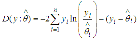 | (20) |
 is the number of events (observed values or counts), n is the number of observations and
  represents the fitted means (predicted values) of the models.For a better model, one must expect a smaller value of the Deviance. Hence the smaller the value of the deviance of a specific model the better the model or the more statistically significant the model becomes.
3.5.2. Akaike’s Information Criterion (AIC)
- Akaike’s Information Criterion (AIC, Akaike, 1973) is a measure of the relative quality of a statistical model for a given data. That is, given a collection of models for a data, AIC estimates the quality of each model, relative to other models. Hence, AIC provides a means for model selection. For any statistical model, the AIC value is computed using the relation;
 | (21) |
3.5.3. Bayesian Information Criterion (BIC)
- Bayesian Information Criterion (BIC) is a criterion for model selection among a finite set of models. It is based in the part on the likelihood function and it is closely related to the Akaike’s Information Criterion (AIC). Mathematically the BIC is an asymptotic result derived under the assumption that, the data distribution is in the exponential family.Let;x=the observed datan=the number of data points in x, the number of observation or equivalently the sample sizek=the number of free parameters to be estimated. For instance if the model under consideration is linear regression, then k is the number of regressors or independent variables, including the intercept.
 the marginal likelihood of the observed data given the model M.
 = the maximized value of the likelihood function of the model M that is
  where
where  is the parameter value that maximizes the likelihood function.Then the formula for the Bayesian Information Criterion (BIC) is given by;
 | (22) |
4. Results and Discussions
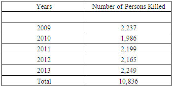
- A review of the road accidents data with respect to the number of persons killed, revealed that there were 79,114 road accidents in Ghana from 2009-2013 which killed 10,836 people. This as a result gives indication that on the average, 15,823 road accidents occur every year and 2,167 lives were lost through road accidents. The table 1 below shows the time in years for which road accidents that resulted in death of people occurred and additionally presents the total number of persons killed in road accidents in road accidents yearly from 2009-2013.
|
4.1. Poisson Regression Model for the Number of Persons Killed in Road Accidents from 2009-2013
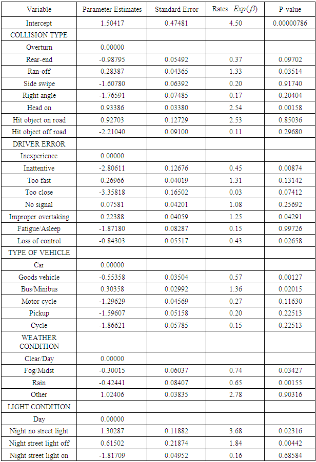
- The table 2 below presents the results on the estimate of the Poisson count regression model for the association of collision type resulting in death, type of vehicle resulting in death, weather condition of occurrence of accident resulting in death, light condition prevailing during accident, and driver error resulting in death. The table contains the parameter estimates, standard errors, death rates and the respective p-values of the various categories of variables used in the model.
|
 | (23) |
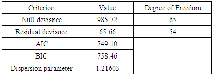
4.1.1. Goodness of Fist Test of the Poisson Regression
- Table 3 below displays the goodness of fit test of the fitted mean Poisson regression model for the number of persons killed in road accidents in Ghana from 2009-2013. This goodness of fit test helps one to determine how quality fit or appropriate the fitted model is as compared to other models.
|
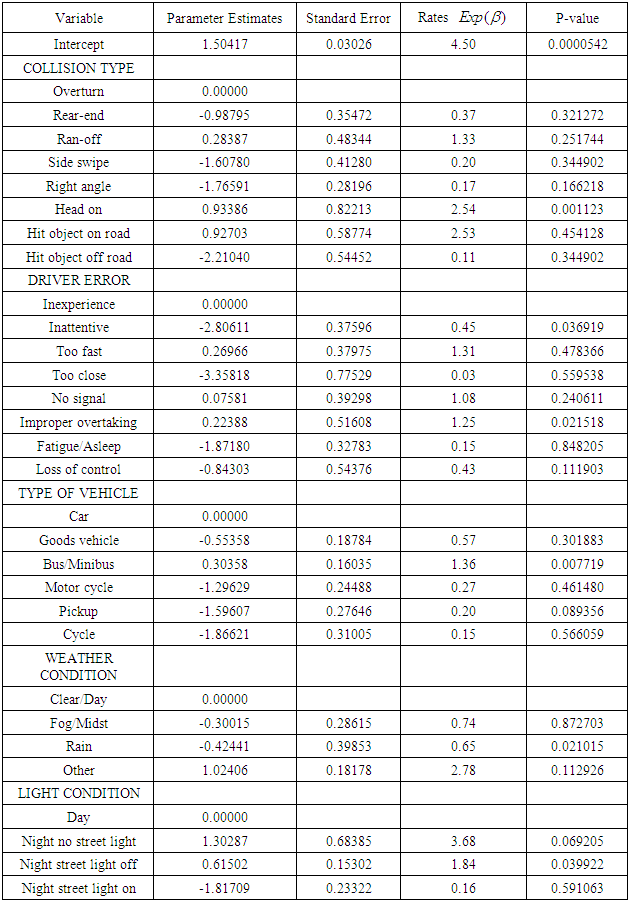
4.2. Negative Binomial Regression Model for the Number of Persons Killed in Road Accidents from 2009-2013
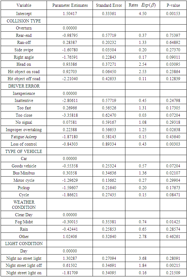
- The table 4 below shows the results of the results of the Negative Binomial regression model with collision type, driver error, and type of vehicle, light condition and weather condition as the independent categorical variables and the number of persons killed as the response variable. The parameter estimates associated with the categorical independent variables were the same as those of the Poisson regression model. As a result the estimated rate of the number of persons killed in road accidents associated with collision type, driver error, type of vehicle, light condition and weather condition remained unaltered. However, the standard errors and the respective probability values p-values changed from one variable to the other.
|
 | (24) |
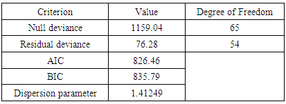
4.2.1. Goodness of Fit Test of the Negative Binomial Regression
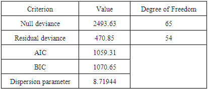
- Table 5 below depicts the goodness of fit test of the fitted Negative Binomial regression model for the number of persons killed as a result of road accidents in Ghana from 2009-2013. This table gives the details of null deviance, residual deviance, AIC, BIC and the dispersion parameter of the model.
|
4.3. Conway-Maxwell-Poisson Regression Model for the Number of Persons Killed in Road Accidents from 2009-2013
- The parameter estimates of the Conway-Maxwell-Poisson model from the table 5 below on the other hand as compared to the Negative Binomial model and Poisson regression model were the same. This as a result give the indication that the estimated rate of death values for the respective variables used in the analysis remains the same as well. However the standard errors and the probability values of the variables involved were changed.
|
 | (25) |
4.3.1. Goodness of Fit test of the Conway-Maxwell-Poisson Model
- The table 7 below indicates the goodness of fit test of the Conway-Maxwell-Poisson regression model for the number of persons killed in road accidents from 2009-2013. This table helps to determine as to whether the fitted model is appropriate or whether the model is quality fit.
|
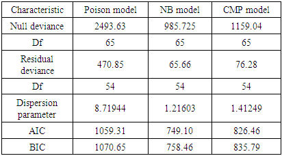
4.4. Model Evaluation and Comparison
- With respect to the table 8 presented above, there is a clear evidence that Negative binomial model performs best and is the best model which best fit the accident data well with respect to the expected number of persons killed in road accidents as compared to the Poisson and the CMP model.This is because in order to select the best model that performs best or best fits with respect to a certain data among other models with the help AIC, BIC or deviance, the criterion set is that, the smaller the value of the AIC or BIC or Deviance the better that model becomes. Hence by comparing the respective values of the AIC, BIC as well as the residual deviance of the Poisson, Negative Binomial and the CMP model from the table 8, it is seen that the Negative binomial has the smallest AIC value of 749.10, BIC value of 758.46 and a residual deviance value of 65.666 as compared those of Poisson and the CMP model.
|
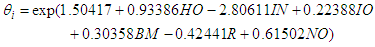
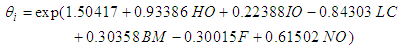 where
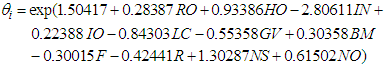
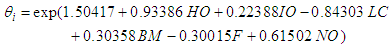
where  represents the expected number of persons killed in road accidents in a particular period of time, HO is Head-on collision, IO is Improper overtaking, LC represents Loss of control, BM is Bus/Minibus, F is Fog/Midst, NO represents Nights with street lights off.
5. Conclusions
- This research work was aimed at examining the efficiency of different statistical models for count data with application to road accidents in Ghana. As a result three (3) statistical models including Poisson, Negative Binomial and Conway- Maxwell-Poisson count regression models were fitted. All the fitted models include significant explanatory variables.Base on the deviances, AIC and BIC of the respective fitted models it appeared that only Negative Binomial model performed best as compared to Poisson and the Conway-Maxwell-Poisson model. The predictors in this model were investigated using their respective p-values and was found out that Head-on collision as collision type, Improper overtaking and Loss of control as driver errors, Bus/Minibus as type of vehicle, Fog/midst as weather condition and Night with street lights off as Light condition were the key predictors or independent variables contributing significantly to the expected number of persons to be killed in road accidents in Ghana.The empirical study of this research work additionally revealed that in the presence of over-dispersion, both the Negative Binomial and Conway-Maxwell-Poisson count regression models are potential alternative to the Poisson count regression model due to its major assumption of equi-dispersion. Thus the Poisson count regression model serves well under equi-dispersion condition whiles both Negative binomial and CMP count regression models serve better whiles the data is over-dispersed.
Appendix
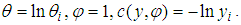
- Derivation of the Poisson RegressionFrom the generalized linear model framework, the exponential family in canonical form is given by the probability function;
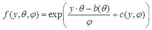 | (1) |
 By taking the exponent and natural log (ln) of the Poisson pdf, we obtain the following;
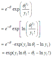 | (2) |
 But
But | (3) |
 | (4) |
 the subject from (11) we obtain;
 | (5) |
 Where
Where  is the observed number of counts (accidents) for
 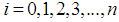 and
and  is the mean or the expected number of counts (persons killed in road accidents) of the Poisson distribution.In the Poisson distribution, the
  was fully determined by a linear combination of
  The Negative Binomial on the other hand adds some unobserved heterogeneity, such that
  is determined by the
  and some unobserved specific random effect called Gamma distributed error
  which is assumed to be uncorrelated with the
  Hence we obtain the following relationships;
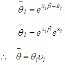 | (6) |
 is defined as the unobserved random effect;
  is the log-link between the Poisson mean and the covariance or independent variables
  and the
  are the regression coefficients.The Negative Binomial is not defined without the assumption about the mean error term and the most convenient assumption is that,
  since this gives
  This is as a result indicates that we have the same expected counts as the Poisson distribution.Since the distribution of the observations is still Poisson with given
  and
and  , we obtain the relation:
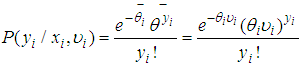 | (7) |
 is unknown.Since
  is unknown,
  cannot be computed and instead there is a need to compute the distribution of
  given
given  only. Hence, to compute
  without conditioning
  , we compute the average of
  by the probability of each value of
  Hence if
  is the probability density function of
  then;
then;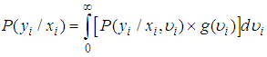 | (8) |
 is a mixing distribution. In the case of the case of the Poisson-Gamma mixture,
  is the Poisson distribution and
  is the Gamma distribution. This distribution has a closed form and as a result leads to the Negative Binomial distribution.In order to solve (17), there is the need to specify the form of the pdf for
  Assuming that the variable
  follows a two-parameter Gamma distribution then we have;
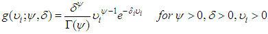 | (9) |
 An interesting thing about this distribution is that,
  which is a convenient assumption indicating that the mean of the Negative Binomial is the same as the Poisson. Also
  By using (7) and (9) to solve (8), we obtain following Negative Binomial model;
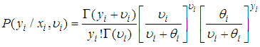 | (10) |
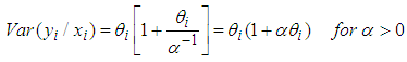
 . But the conditional variance differs from that of the Poisson distribution;
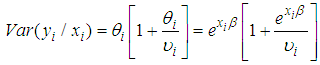 | (11) |
 and
and  are both positive from (11), the variance automatically exceeds the conditional mean. This as a result increases the relative frequency of low and high counts. There will be more parameters than observations since the variances remain undefined if
  varies by observation. The typical assumption is that
  is the same for the observations (counts) that is;
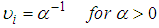 | (12) |
 | (13) |
 | (14) |