1. Introduction

Data analysts are frequently faced with the missing value problem. Missing values may occur for various reasons which may include poor record keeping, lost records, technical error, collecting data at irregular times, etc., ([1], [2]). In addition, a peculiar case can arise when one may be interested in determining the likely value of a variable of interest at a time that may not coincide with a particular measurement or observation [3]. These can result in one or several observations missing.

These missing values must be accounted for since missing values have negative effects on the modeling of the data [4]. There are many ways of handling missing values. The common approach is to use imputation techniques. This involves using a substitute value to replace the missing observation as in [5]. According to [6], imputation broadly comprises several techniques that have been developed to compute missing values. These techniques may employ strategies such as mean substitution and artificial neural networks approach. It may also involve the use of appropriate statistical prediction or forecasting models such as regression, time series models, and Markov chain and Monte Carlo methods.

Estimation of missing values for bilinear time series has been done for a particular order of the bilinear time series BL (1, 0, 2, 0) by [4]. They used estimating functions criterion to derive the estimates of missing values. Other studies have also been done to estimate missing values for pure bilinear time series when the innovation sequence has the GARCH distribution [7]. Still the same authors have estimated missing values for pure bilinear time series when the innovation sequence has the normal distribution [8]. [9] also estimated missing values for bilinear time series for the pure bilinear case when the innovation sequence has the student-t distribution. They found that the estimates of the missing values were equivalent to a one–step-ahead forecast. Further, [10] used the linear interpolation criterion to estimate missing values for the BL (p, 0, p, p) when the error term follows the normal distribution.

The distribution of interest in this study is the student-t distribution. This distribution is characterized by long tails and is suitable for modeling financial data which is known to be highly skewed. There is no evidence to show that optimal linear interpolation approach based on the dispersion error has been used to estimate missing values for bilinear BL (p, 0, p, p) with student-t distribution.

1.1. Identification of Bilinear Time Series Models

Given a time series data, the first step in the identification process of bilinear time series model is to test whether the data can be modeled either as a linear time series or belongs to the broader class of nonlinear time series models. This involves testing a null hypothesis that the data is linear. This can be done using one of the statistical tests of linearity ([11]; [12]). If the null hypothesis is rejected then the data can be appropriately modeled by a nonlinear series model and a bilinear model is one of the candidate models to be considered ([13]; [14]). If the data is nonlinear then the second step is used.

The second step in the identification process is to determine the class of the nonlinear models to which the data belongs. This involves the use of moments and cumulants. It has been noted that BL (p, 0, p, 1) and ARMA (p, 1) models have similar second order moments and hence these moments cannot be conclusively used in the identification of the bilinear time series models [15]. Consequently, it is imperative to use higher order moments. The higher moments are known to satisfy the Yule-Walker type difference equations ([15], [16]). Thus these equations could be used for model identification of the bilinear time series models. The difference between the moments of bilinear time series and those of the other nonlinear time series models is that the higher order moments of a bilinear time series (including the fourth moments) decay slowly as the lag tends to infinity. However, the fourth moments of the other nonlinear time series models do not behave in a similar manner.

After determining that the data is bilinear, then the order of the model is computed using canonical correlation analysis carried between the linear combinations of the observations and linear combinations of higher powers of the observations.

For some super diagonal and diagonal bilinear time series, the third order moments are not equal to zero. This pattern of nonzero moments can be used to discriminate between white noise and the bilinear models and also between different bilinear models [16]. Using the patterns presented in a table of third order moments, one can easily distinguish bilinear models from pure ARMA or mixed ARMA models. Third order moments may also be useful in detecting non-normality in the distribution of the innovation sequence.

This technique of model identification can be extended to more general bilinear models provided that difference equations for higher order moments and cumulants can be obtained [15].

1.2. Estimation of Parameters of the Bilinear Time Series Models

Several estimation techniques have been proposed for the estimation of the parameters of the bilinear time series in the literature. Most of them deal with particular classes of the bilinear time series models [9]. [13] proposed two methods for the estimation of the model parameters of a bilinear time series models, namely the use of Newton Raphson technique and the Marquart Algorithm. He applied both methods to the estimation of the parameters of a bilinear time series model identified for sunspost and seismology data. Secondly, he proposed estimation of the parameters using maximum likelihood method. More recently [18] proposed a generalized autoregressive conditional heteroskedasticity- type maximum likelihood estimator for estimating the unknown parameters for a special bilinear model. They showed that their proposed estimator was consistent and asymptotically normal under only finite fourth moment of errors. [19] proposed the use of covariance estimates based on the least squares method on the parameters of the bilinear model BL (p, 0, p, 1). [20] estimated the parameter of the simple diagonal bilinear model BL (0, 0, 1, 1) using the least squares method.

2. Literature Review

2.1. Student-t Distributions

Most of the data encountered in practice show departure from the linearity and thus may be modeled by nonlinear time series models [21]. These models have innovations that can adequately be described by student-t, ARCH and stable distributions. For financial data, models with the student-t distribution play an important role in modeling. The student-t distribution can be integrated with other distributions such as GARCH to produce even better models. For example, GARCH (1, 1) model with student-t distribution is able to reproduce the volatility dynamism of financial data. Given a model, specification for log of return disturbances can be modeled using either the student-t distribution or the normal distribution. However, the student-t distribution is particularly useful since it can describe the excess kurtosis in the conditional distribution that is found in financial time series unlike the models with normal innovations (Owili, 2015c).

[22] focused on the bilinear time series model with GARCH innovations (BL-GARCH). It has an important property that it can take into account explosions and related volatility features of non-linear time series. The most common model used in financial data is the BL-GARCH (1,1) model and may be used in practical applications with either the normal, the student-t or GED noises.

2.2. Empirical Studies on Bilinear Models

The bilinear time series models find applications in many areas such as hydrology, economics and finance. Since it is a complicated model, only specific classes of the bilinear models have been studied. For example, [13] considered model BL (p, 0, p, q); [11] studied the asymptotic behavior of the correlation function for the simple bilinear model BL (0, 0, 1, 1); [23] and [24] studied the model BL (1, 0, 1, 1); [25] considered the model BL (0, 0, 1, 1). [26] estimated the coefficients of a bilinear model BL (1, 0, 1, 1) using the maximum likelihood method. [24] claimed that estimating bilinear models is quite challenging.

It can be seen from the literature that several studies on inferences based on bilinear time series models have been done. These include model identification, determining conditions necessary for stationarity and invertibility and estimation of the parameters of the bilinear time series models. On missing value, Owili, Poti and Orawo (2015) only studied pure bilinear model BL (0, 0, p, p). No study has been done on the general bilinear model BL (p, 0, p, p). Therefore, the aim of this study was to derive estimators of missing values for BL (p, 0, p, p) using the optimal linear estimation approach of [28].

2.3. Estimation of Missing Values using Linear Interpolation Method

Suppose we have one value missing out of a set of an arbitrarily large number of n possible observations generated from a time series process Let the subspace be the allowable space of estimators of based on the observed values 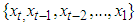i.e., = sp where n, the sample size, is assumed large. The projection of onto (denoted ) such that the dispersion error of the estimate (written disp is a minimum would simply be a minimum dispersion linear interpolator. The missing value is estimated as

(1)

where is the estimate obtained from the model based on the previous lagged observations of the data before the point m, the missing data point and x_m the missing value, the coefficients (k=1, 2,..k-m) are to be estimated by minimizing the dispersion error (disp ) given by equation (1) as in [28].

3. Research Methodology

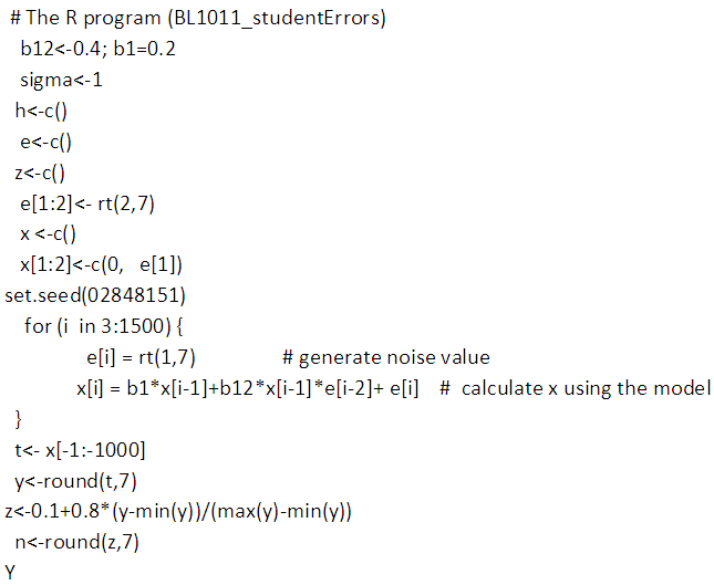
Data was simulated from the general bilinear time series models BL (1, 0, 1, 1) with student-t innovations using R statistical software. A program code in R was used. 100 samples of size 500 each were generated and missing artificial points were created at data point 48, 293 and 496. These points were selected at random. Data analysis was done using the following software: Microsoft Excel, TSM, R and Matlab7. The mean squared error (MSE) and mean absolute deviation (MAD) were used as performance measures.

4. Results

4.1. Derivation of the Missing Values for Bilinear Time Series Models with Student-t Innovations

Estimates of missing values for BL (p, 0, p, p) bilinear time series models whose innovations follow student-t distributions were derived based on minimizing the h-steps ahead dispersion error. Two assumptions were made in the process of the derivations. The first one was that the time series data is stationary. Secondly, the higher powers (of orders greater than two or products of coefficients of orders greater than two) of the coefficients are approximately negligible. This was consequence of the result of the first assumption.

4.1.1. Estimating Missing Values for BL (1, 0, 1, 1) with t- Errors

The bilinear model BL (1, 0, 1, 1) with t- errors is expressed as

The missing value is obtained using theorem 4.1

Theorem 4.1

The optimal linear estimate for missing value for

BL (1, 0, 1, 1) with student errors is given by

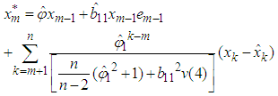Proof

The stationary BL (1, 0, 1, 1) can be expressed as

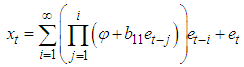The h-steps ahead forecast is given by

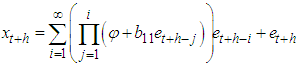and the h-steps ahead forecast error is given by

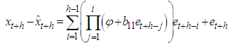(3)

Substituting equation (3) in equation (1), we obtain

(2)

Simplifying the terms RHS of equation (2), we obtain

where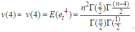

Hence equation (2) becomes

(3)

Differentiating equation (3) with respect to the coefficients, we get

The optimal linear estimator of denoted that minimizes the error dispersion error is

4.1.2. Estimating Missing Values for Bilinear Time Series Model BL (p, 0, p, p) with Student-t Innovations

The pure bilinear time series model BL (p, 0, p, p) with student t errors is

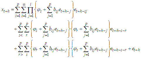
The missing values can be estimated using theorem 4.2.

Theorem 4.2

The optimal linear estimate for one missing value x_m for the general bilinear time series model BL (p, 0, p, p) with student t-errors is given by

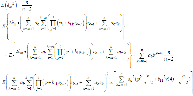
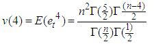
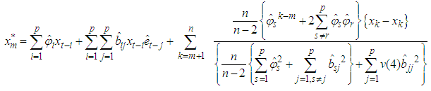Where v(4) is the fourth moment of the data given.

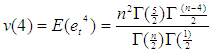Where v(4)=kurtosis*(variance)^2.

Proof

The stationary bilinear time series model BL (p, 0, p, p) is of the form

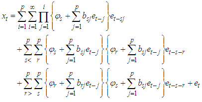(4)

The h steps ahead forecast based on equation (4) is given by

(5)

Or

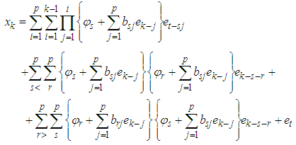The forecast error is

(5)

Substituting equation (5) in equation (1) and simplifying, we obtain

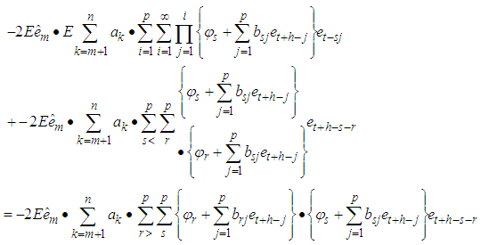First term

Second term

Third term

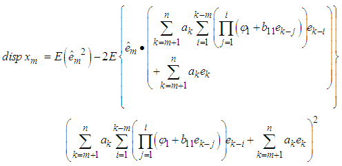
This simplifies to

(6)

where

Differentiating equation (6) with respect to , we have

Solving for we get

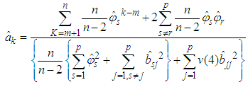Corollary

For p=1, we have the bilinear model BL (1, 0, 1, 1). The best linear estimate is given by

4.2. Simulation Results

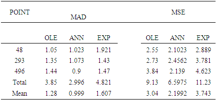
In this section, the results of the optimal linear estimator, artificial neural networks and exponential are given in table 1.

Table 1. Efficiency Measures for BL (1, 0, 1, 1) with student-t innovations

From table 1, it can be concluded that ANN estimates most efficient (MSE=2.1992) for the different missing data point positions followed by OLE estimates (MSE=3.04). This is in contradiction to the results obtained for pure bilinear time series model BL (0, 0, 1, 1) by [9].

5. Conclusions

In this study we have derived estimates for missing values for the bilinear time series model BL (p, 0, p, p) with student-t innovations. The study found that ANN estimates were the most efficient compared to both the OLE and EXP. Further the estimates of the missing values were found to be dependent on the observations before and after the missing value point.

Appendix

Appendix A: Program Codes used in simulation