Morteza Marzjarani
NOAA, National Marine Fisheries Service, Southeast Fisheries Science Center, Galveston Laboratory, Galveston, USA
Correspondence to: Morteza Marzjarani, NOAA, National Marine Fisheries Service, Southeast Fisheries Science Center, Galveston Laboratory, Galveston, USA.
| Email: |  |
Copyright © 2016 Scientific & Academic Publishing. All Rights Reserved.
This work is licensed under the Creative Commons Attribution International License (CC BY).
http://creativecommons.org/licenses/by/4.0/

Abstract
The issue of handling categorical along with continuous variables in linear models is always interesting and at the same time challenging. In this paper, a general linear model is extended to include both categorical and continuous predictors. Second order terms including interactions of categorical and continuous variables are discussed. Relations are defined, which map categorical variables onto continuous ones. A special case of such relation is where the levels of categorical variables are nested within the continuous variables hereafter called a “nested” model. The resulting models are then applied to estimate shrimp effort in the Gulf of Mexico for the years 2007 through 2014. A comparison of the results from each of the models is presented in the paper.
Keywords:
General linear models, Relations, Interactions
Cite this paper: Morteza Marzjarani, Higher Dimensional Linear Models: An Application to Shrimp Effort in the Gulf of Mexico (Years 2007-2014), International Journal of Statistics and Applications, Vol. 6 No. 3, 2016, pp. 96-104. doi: 10.5923/j.statistics.20160603.02.
1. Introduction
In building a model for a given data set(s), it is always interesting and sometimes necessary to include the impact of interactions between or among predictors in the model. Adding such interaction terms to a model can significantly increase the understanding of the relationships among the variables in the model and create more hypotheses, which can be tested. Analyzing interactions or more generally, relationships among continuous predictors, is a straightforward issue, but the problem becomes much more complex when categorical predictors are added to the models. Review of current literature on this issue shows that such relationships have been studied up to the analysis of variance and measuring interactions through some contrasts. However, the issue of estimation or prediction in such cases has yet to be fully addressed in the literature. The interaction between categorical and continuous variables is somewhat easy to handle so long as the categorical variables are binary or in a not too favorable way, the continuous variables can also be converted to binary categorical variables. Based on my review of the literature, none of the papers related to this topic have been published in the peer reviewed literature. See Benoit (2010), Templin (no date) for example. In this paper, I propose to convert the categorical variables to proper dummy codes, test interactions in the usual way, and use the results to estimate/predict the response variable. I also propose to set up relations (functions as special cases) which map categorical variables onto continuous variables or predictors. A special case of such relation is the simple mapping of the categorical variables onto the continuous ones known as “nested” models. For the purpose of fishery management, the Gulf of Mexico (GOM) region is divided into twelve SEDAR1 zones (Figure 1a) and twenty-one statistical subareas (Figure 1b). Each SEDAR zone consists of a two-digit number, the first digit stands for "area", a number between 1 and 4 inclusive, and the next for "depth", a number between 1 and 3 inclusive.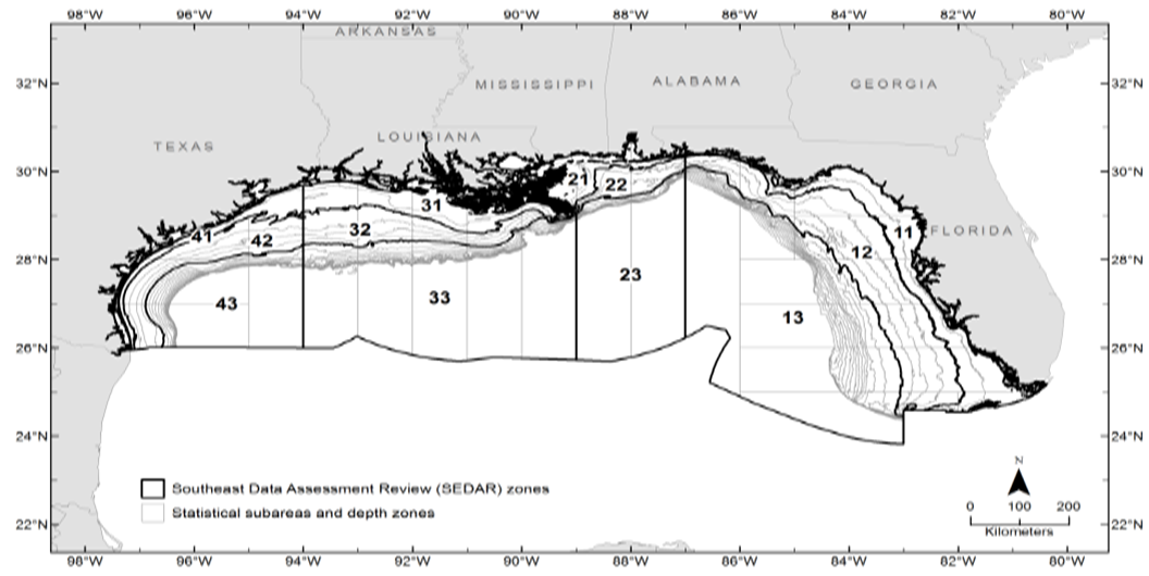 | Figure 1a. Southeast Data Assessment Review (SEDAR) zones and statistical subarea and depth fathom zones in the Gulf of Mexico |
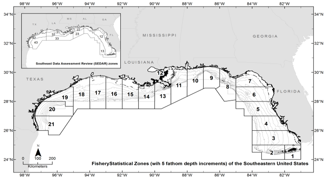 | Figure 1b. The Gulf of Mexico is divided into twenty-one statistical subareas (1-21) as shown |
The data files for this study, primarily consisted of three files (Analyst, AllocZoneLands, and Vessel) for each year. In the following, each file is described briefly.
1.1. Definition and Composition of Data Files
1.1.1. Analyst File (years 2007-2014)
The analyst file is the legacy name of the analyst final table in the Gulf Shrimp System (GSS). This table contains the state trip ticket and port agent interview data for the Gulf of Mexico shrimp fishery. The GSS began in the late 1950s and contains shrimp landings (pounds) caught in the US Gulf of Mexico. There are several fields in this file. Some fields of interest to this study were: USCG vessel number (vessel), port (port), catch unload date (edate), statistical subarea, depth fathom zone, catch weight (pounds), and price per pound (priceppnd). After all the necessary corrections in the data sets collected from dealers and port agents are made, the Analyst file is generated via software owned by the National Marine Fisheries Service (NMFS).
1.1.2. AllocZoneLands file (years 2007-2014)
The AllocZoneLands file is generated by the electronic logbook (ELB) analysis software. This file is the final output where landings reported in the GSS are matched to fishing effort reported by the ELB. The file contains an instrument identifier, the end date of the trip (edate), with pounds (lands), and effort (towdays-days fished) placed in per zone (a four-digit number where the first two digits are statistical subarea and the next two digits are depth fathom zone).
1.1.3. Vessel File
The vessel file is a combination of the ELB assignment data table and vessel characteristics data from the United States Coast Guard data tables. The assignments table contains the instrument device identifier (ELB) and the USCG documentation number (vessel). This is joined to the USCG data to provide additional information like horsepower and vessel length (length).
2. Method
In order to develop a model for the shrimp effort estimation several steps had to be taken. The first step was to convert each Analyst file (2007 through 2014) into a new file called “Trips” based on the vessel id number, edate, and port. In addition, the weighted average price per pound (hereafter called wavgppnd) was computed and assigned as the price per pound for the corresponding trips in the Trips files. A non-monotone imputation method (Rosenbaum and Rubin, 1983), Rubin (1987), Schafer (1997), and Yuan (2011) was used to fill in a few missing price per pound or pounds in the corresponding fields. In this paper, I identified two patterns: Monotone and Non-monotone (Arbitrary). A data set is said to be in monotone pattern if a triangle consisting of cells with missing value can be formed in the lower right corner (Figure 2a). In other words, if in the i-th row, Yj is missing, all subsequent values must also be missing. An arbitrary (non-monotone) pattern does not follow any specific missing pattern (Figure 2b). It was important to recognize the missing patterns before imputation.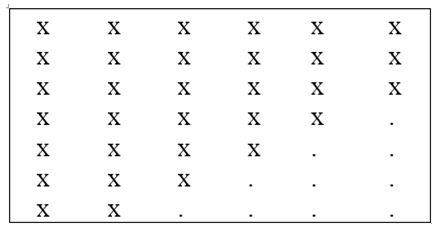 | Figure 2a. A monotone pattern |
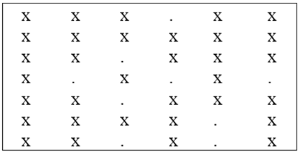 | Figure 2b. An arbitrary pattern |
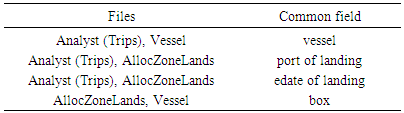
Next, the resulting individual Trips file was merged to create a large file (hereafter called AllTrips) with 435,094 records or trips, then merged with the individual AllocZoneLands files creating another large file hereafter AllocZoneLandsAll file with 65,530 records. The following step was to match the three data files AllTrips, AllocZoneLandsAll, and Vessel based on the common fields listed in Table 1 to create a file called “Match” with 61,232 records each consisting of 18 variables.Table 1. Common fields used in creating the Match file
 |
| |
|
Since area and depth were considered as two independent variables to be included in the model, the zone field (see AlloczoneLands file) in the newly created Match file was split into two fields: statistical subarea (a number between 1 and 21) and depth fathom zone (a number between 1 and 12). By using the conversion given in Figure 3, these two fields were then converted to area (a number between 1 and 4) and depth (a number between 1 and 3) representing the levels of the two categorical variables area and depth in the Match file respectively. 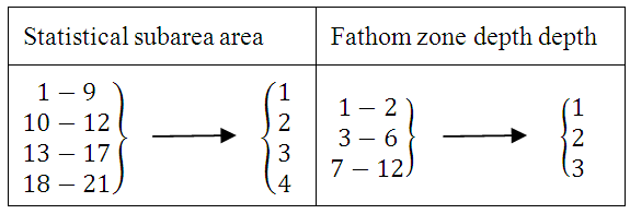 | Figure 3. Conversion of statistical subareas (1 through 21) and depth fathom zones (1 through 12) into area (1 through 4) and depth (1 through 3) respectively |
Similarly, the calendar year was also placed into a three-level categorical variable, trimester (January-April, May-August, and September-December). The Match file then was run through the statistical models described below and parameters of the models were estimated. To estimate fishing effort (towdays), the Analyst files again were converted to trips using a similar approach deployed earlier but adding the SEDAR zone as another factor marking the end of a trip. Also, this field was split into area and depth for the two categorical variables area and depth included in each model. Since the vessel length was included as a continuous variable in the model, there was a need for adding this field to the Trips file. Several sources including the Vessel file (s) and the United States Coast Guard site were used to fill this field. A monotone imputation method (Rosenbaum and Rubin, 1983), Rubin (1987), Schafer (1997), and Yuan (2011) was deployed to fill the remaining missing vessel lengths. Finally, the resulting file with 147,037 records or trips was used to estimate effort generated by each model.
2.1. The Model
The purpose of this study was to extend a general linear model to include higher order terms. I began with a model consisting of first order terms of all continuous and categorical variables and the second terms of continuous variables as follows: 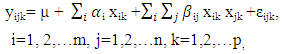 | (2.1) |
In this model,  is the overall mean,
  is an iid (independently identically distributed) normally distributed random variable with mean 0 and standard deviation σ2 (that is, a homoscedastic model).
  and
and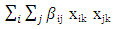 represent the first and second order terms of continuous variables length, lnlbs (natural logarithm of variable pound), and wavgppnd. Model (2.1) was written again below but this time the second terms were extended to include the categorical variables area, depth, trimester, year and their interactions.
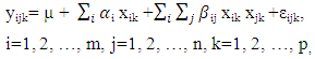 | (2.2) |
In the next step, the model was further developed to include relations among continuous and categorical variables. In general, a relation can be defined on two or more variables. Such a relation can be deployed as many-to-many, one-to-many, or many-to-one (function).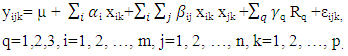 | (2.3) |
where 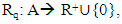 R+ is the set of positive real numbers, and A is a set consisting of some categorical variables. Each term in the sum
  is a relation along with its corresponding unknown parameter, which is to be estimate. More precisely, here
 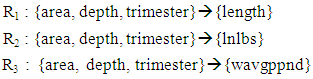 | (2.4) |
Each of these relations can take different forms. Defining such relation depends on the knowledge of the experimenter, but the more challenging part is the implementation of it. Even a slightly wrong implementation or a slightly improper relation would result in a totally different estimate for the response variable. Out of numerous possibilities for a many-to-one relation, one is of special interest where levels of the categorical variables are nested within each continuous variable, hereafter called Model (2.3) (to keep the model numbers in sequence). Figure 4 demonstrates a very simple case of a relation known as nested (or hierarchical) model where categorical variables are nested within continuous variables.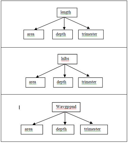 | Figure 4. Categorical variables are nested within continuous variables |
Nesting of categorical variables within another categorical variable are discussed in the literature (Kriwoluzky and Stoltenberg, 2015), (Jung et al., 2008), (Yan et al., 2012). It should be mentioned that the definition of nested model used here is a bit more general than that used in these references. In this paper, a categorical variable is said to be nested within another variable (continuous or categorical) if its levels are mapped onto the second variable via a mathematical relation.The normality assumption of the error term was approximately satisfied (76%, 96%, and 99% for 1-sigma, 2-sigma, and 3-sigma respectively). In order to test and select the significant parameters listed in models (2.1) through (2.3) two different and independent approaches were deployed.
2.1.1. Approach 1
In this approach, the usual method of testing the hypotheses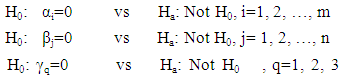 | (2.5) |
was used, parameters were tested and significant ones (p-value < 0.05) were included in the models. Due to a large number of significant parameters, the list was not included in this research.
2.1.2. Approach 2
In this totally independent and different approach, a selection method hereafter called “Selection” with backward elimination was used to choose a proper model with the commonly used significant levels 0.15 and 0.08 for entering into or removing predictors from the model respectively using either the optimum value for Adj. R-Sq or Mallows' Cp, Mallows (1973) and Gilmour (1996) for the selection of the model. In this paper, I deployed the commonly used form of Adj. R-Sq appearing in most introductory books in statistics. The Mallows’ Cp is an alternative criterion for selecting a model and it is defined as: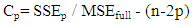 | (2.6) |
where SSEp is the error sum of squares with p predictors in the model, n is the sample size, and MSEfull is the error mean square for the full model. The Selection method stops when Cp is small or it is close (preferably less than or equal to) the number of parameters in the model. There are several other criteria one can use to select a model. As mentioned above, in this research, two of these criteria, Adj. R-Sq and Mallows’ Cp were used.
3. Analysis/Results
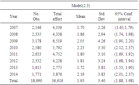
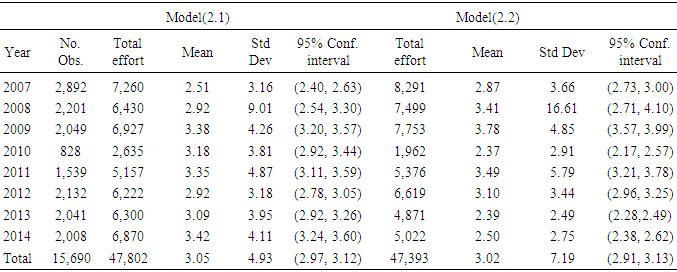
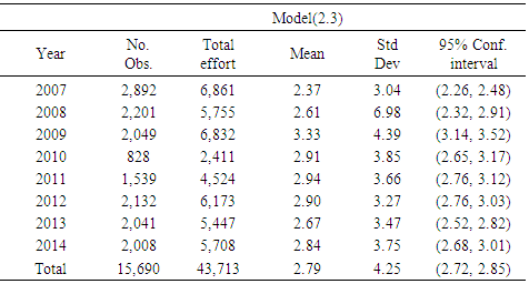
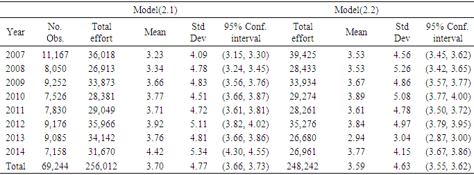
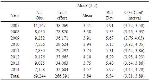
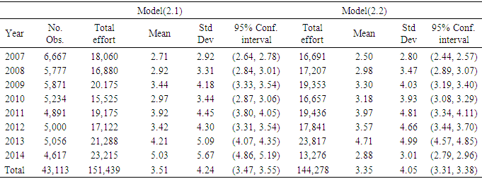
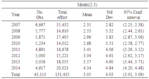
In this study, the relation was assumed to follow Figure (4), that is, a hierarchical model. After applying the models (2.1) through (2.3) the following results were obtained. Due to a very large number of significant parameters especially in cases of models (2.2) and (2.3), these parameters were not listed in this research. Tables 2 through 5 display the shrimp efforts produced by models (2.1) through (2.3) by area along with some statistics of interest per year for areas 1, 2, 3, and 4 (see Method section). In these tables, the “Total effort” column refers to the total days fished per year.Table 2. Shrimp effort generated by Models (2.1) through (2.3) in Approach 1 for years 2007 through 2014 in area 1 in the Gulf of Mexico
 |
| |
|
Table 2. Continued. Shrimp effort generated by Models (2.1) through (2.3) in Approach 1 for years 2007 through 2014 in area 1 in the Gulf of Mexico
 |
| |
|
Table 3. Shrimp effort generated by Models (2.1) through (2.3) in Approach 1 for years 2007 through 2014 in area 2 in the Gulf of Mexico
 |
| |
|
Table 3. Continued. Shrimp effort generated by Models (2.1) through (2.3) in Approach 1 for years 2007 through 2014 in area 2 in the Gulf of Mexico
 |
| |
|
Table 4. Shrimp effort generated by Models (2.1) through (2.3) in Approach 1 for years 2007 through 2014 in area 3 in the Gulf of Mexico
 |
| |
|
Table 4. Continued. Shrimp effort generated by Models (2.1) through (2.3) in Approach 1 for years 2007 through 2014 in area 3 in the Gulf of Mexico
 |
| |
|
Table 5. Shrimp effort generated by Models (2.1) through (2.3) in Approach 1 for years 2007 through 2014 in area 4 in the Gulf of Mexico
 |
| |
|
Table 5. Continued. Shrimp effort generated by Models (2.1) through (2.3) in Approach 1 for years 2007 through 2014 in area 4 in the Gulf of Mexico
 |
| |
|
To avoid redundancy, Approach 1 was selected and efforts generated by the models in the approach were categorized by area. Considering each area individually, in areas 1, 2, and 3, year was significant, but model was not. In area 4 neither year nor model was significant.Intuitively, since area 3 generally generated higher effort, one can conclude that the four areas should show a significant difference. Analysis showed that in fact areas 1 through 4 were statistically different, but no significant differences were observed among years. A multiple comparison method was used to determine which pair (s) of effort means was (were) causing the impact of area to be significant. Out of few multiple comparison methods, Fisher’s Least Significant Difference, LSD, Hayter (1986) and Tukey’s Studentized Range test or known as HSD (Honestly Significant Difference), Tukey (1949) were deployed here. 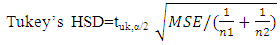 | (2.8) |
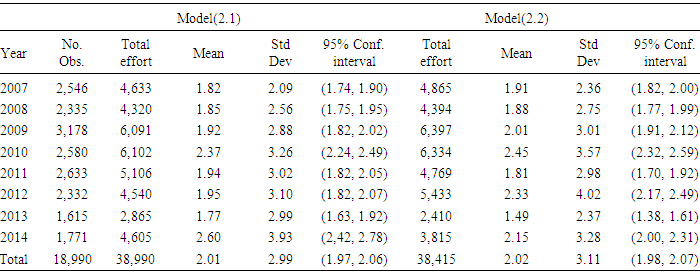
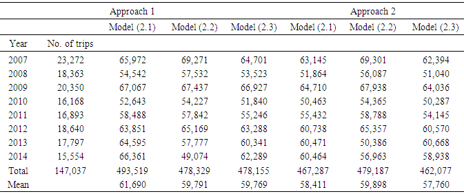
where tuk,α/2 is from Tukey’s studentized table based on α (significance level), n1 and n2 are the mean sample sizes, and MSE is the pooled variance (see an introductory book in statistics for definition). Tukey’s HSD is very similar to Fisher’s LSD except the values of tuk have been computed to take into account all the inter-dependencies of the different comparisons. Analysis showed that based on the calculated Tukey’s HSD=5,853.6, 3,989.6, and 3,018.4 or Fisher’s LSD= 4,367.4, 2,976.7, and 2,252 with α=0.05 for efforts generated by models (2.1) through (2.3) respectively, three distinct categories A, B, and C were recognized. Area 3 and area 4 were placed in two distinct categories A and B, and areas 1 and 2 were placed in the last category C. That is, there was no significant difference between the mean efforts in areas 1 and 2, but area 3 and area 4 were statistically different from each other and from areas 1 and 2. Table 6 shows the efforts produced by model (2.1) through (2.3) for both Approach 1 and Approach 2. There is no significant difference among the models in this table (p-value>0.05).Table 6. Number of trips and effort generated per year for models (2.1) through (2.3) within approach
 |
| |
|
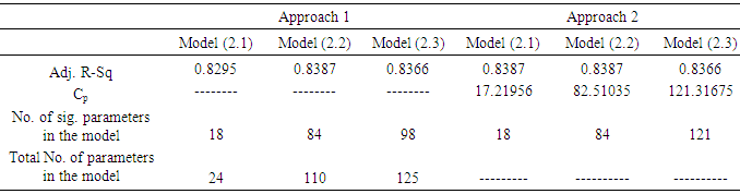
Table 7 displays the adjusted R-Sq, CP, the number of parameters and also the number of significant parameters left in the model.Table 7. Adj. R-Sq, Cp, and number of parameters for models (2.1) through (2.3) within Approach1 and Approach 2 (including levels of categorical variables in Approach 1 with the last level of each as reference)
 |
| |
|
In Approach 2, the selection process stopped revising the model when the optimum value for the R-Sq was reached or when the CP was close to the number of parameters in the model.
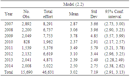
4. Discussion
The goal of this research was to develop a more complex model by including higher order terms such as interactions for the shrimp effort estimation in the Gulf of Mexico. Three possibilities for the model were considered along with two different approaches. At the first attempt, in the second approach, year was included in the relations along with area, depth and trimester. While attempting to estimate the effort, the file became large (over 800 parameters in the model). Subsequently, year was removed from the relations, but still was implemented as a categorical variable in the all models.The standard deviation in area 2, year 2008, was unusually large. Further review showed that there was a record in the raw Analyst file with 1,397,516 pounds of shrimp reported. Although very high, considering the other related fields in this file, this number seemed reasonable. The most likely possibility is that, this could have been the result of putting several records together and reporting it as one record. Fortunately, this record did not contribute to the Match file, and therefore, the parameter estimates were not affected by this record. A part of Table 3 was reproduced after removing this record completely (Table 8). This resulted in a reduction of 722 towdays.Table 8. Reproduced: Shrimp effort generated by Models (2.1) through (2.3) in Approach 1 for years 2007 through 2014 in Statistical Area 2 in the Gulf of Mexico after removing the record reported with high pounds
 |
| |
|
Alternatively, the value in this field was assumed missing and an MCMC imputation method (Yuan, 2011) was used and the hypothetically missing value was estimated at 4,551.87 resulting in the reduction of 463 towdays. Not surprisingly, using the optimum value for either Adj. R-Sq or Cp to select the model produced the same results. Generally, one of selection criteria, Adj. R-Sq or Cp (or others) is sufficient for selecting a model.As table 6 shows, the mean efforts generated by Approach 1 and Approach 2 are relatively close (the range is 3,930). Also, according to Table 7 Adj. R-Sq values for Models (2.2), and (2.3) under Approach 1 and all models under Approach 2 were virtually the same. One interpretation of these could be the fact that the models were selected properly and any of these models could be used as a candidate for the effort estimation at this time.
5. Conclusions
In this research several models and methods were deployed and efforts were estimated. Even though models and methods were completely independent of each other, the results were within a striking distance, which could be interpreted as the proper selection of the models. A method for prediction or estimation of the response variable in the presence of categorical variables was proposed. In addition, a general linear model was extended to include a relation (s), which could be implemented in special cases such as nested models. It is very important to make sure that the relations among independent variables are defined and implemented correctly. Familiarity with mathematical relations, modeling, and the data set(s) are essential to the accuracy of both definition and implementation of such relations. Definition of nested models appearing in literature was extended to include the mapping of categorical variables onto the continuous or categorical variables. The findings in this research will provide methods for estimation/prediction in linear models in the presence of both continuous and categorical variables and will provide a more general and flexible method for dealing with relations (interaction as a special case) among such predictors.1The term SEDAR stands for South East Data, Assessment, and Review is the cooperative process established in 2002 by which stock assessment projects are conducted in NOAA Fisheries' Southeast Region. SEDAR was initiated to improve planning and coordination of stock assessment activities and to improve the quality and reliability of assessments (http://sedarweb.org).The views expressed in this article are the author's own and do not necessarily represent those of NOAA or its affiliates.
References
| [1] | Benoit, K. (2010). Multiple regression with interactions, PO7001. Quantitative Methods I, 1-64. Available: http://www.kenbenoit.net/courses/quant1/Quant1_Week10_interactions.pdf. (March 3, 2016). |
| [2] | Gilmour, S. G. (1996). The interpretation of Mallows' Cp-statistic. Journal of the Royal Statistical Society, Series D 45 (1): 49–56. |
| [3] | Hayter, A. J. (1986). The maximum familywise error rate of Fisher's least significant difference Test. Journal of the American Statistical Association, 81,1000-1004. |
| [4] | Kriwoluzky, A. and Stoltenberg, C. (2015). Nested models and model Uncertainty. Scand. J. of Economics, 1-29. |
| [5] | Jung, B. C. and Khuri, A. I. and Lee, J. (2008). Comparison of designs for the three-fold nested random models. Journal of Applied Statistics, Vol. 35, 701-715. |
| [6] | Mallows, C. L. (1973). Some comments on CP, Technometrics, 15 (4), 661–675. |
| [7] | Rosenbaum, P. R. and Rubin D. B. (1983). The Central role of the propensity score in observational studies for causal effects. Biometrika, 70, 41–55. |
| [8] | Rubin, D. B. (1987). Multiple imputation for nonresponse in surveys. New York, John Wiley & Sons, Inc. |
| [9] | Schafer, J. L. (1997). Analysis of incomplete multivariate data. New York, Chapman and Hall. |
| [10] | Templin, J. (no date). Continuous and categorical independent variables -I: Attribute-treatment interaction; comparing regression equations, 1-45. Available: http://jonathantemplin.com/files/regression/epsy581s05/epsy581_19.pdf. (March 3, 2016). |
| [11] | Tukey, John (1949). Comparing individual means in the analysis of variance. Biometrics 5 (2), 99–114. |
| [12] | Yan, J. and Aseltine, R. H., and Harel, O. (2012). Comparing regression coefficients between nested linear models for clustered data with generalized estimating equations. Journal of Educational and Behavioral Statistics. Vol. 38, no. 2, 172-189. |
| [13] | Yuan, Y. (2011). Multiple imputation using SAS software, Journal of Statistical Software, Vol. 45, Issue 46, 1-25. |

 Abstract
 Reference
 Full-Text PDF
 Full-text HTML