1. Introduction

Childhood undernutrition has severe adverse growth effects on a child. An undernourished child is more likely to be sick and die [1]. In sub-Sahara Africa, this problem often leads to more than 30% of deaths in children below five years annually [2]. Undernutrition is also a strong indicator of retarded growth [3], impaired cognitive and behaviour development [5], poor school performance, and lower working capacity [4]. If not corrected, it can slow down economic growth and increase poverty levels. Furthermore, it can prevent a nation from meeting its full potential through loss in productivity, cognitive capacity and increased cost in health care [5]. The indicators of undernutrition are stunting, wasting and underweight.

The reduction of childhood malnutrition is the United Nations Millennium Development Goal (MDG) number 1 [2, 4], which aims at halving the proportion of children suffering from hunger by 2015. In addition, it has direct impact on the MDG number 4 which aims at reducing the under-five mortality rate by two-thirds by 2015 [2, 4]. In order to attain both MDG1 and MDG4, various malnutrition intervention projects have ever been launched in Namibia since 2007. However, no appropriate in-depth evaluation has been made to statistically understand the socio-demographic determinants and spatial variation of severe childhood malnutrition in Namibia. Research has shown that the prevalence of childhood stunting in Namibia is currently about 24% [6]. The main aim of this study was to assess socio-demographic determinants and geographical variation of severe childhood stunting prevalence in Namibia using spatial quantile regression models.

Spatial models have previously been used to analyse childhood stunting in most sub-Sahara African countries other than Namibia [8, 9]. Unfortunately, these have emphasized on modelling mean regression instead of quantile regression. Modelling malnutrition using quantile regression is more appropriate than using mean regression with extensive literature examples [10, 12, 19, 25-30], in that it provides flexibility to analyse the determinants of malnutrition corresponding to quantiles of interest either in the lower tail (say 5% or 10%), upper tail (say 90% or 95%) or even median (50%) of the distribution rather than only analysing the determinants of mean distribution. When modelling malnutrition, it makes more sense to model severe responses rather mean responses [10, 12, 19, 25-30]. For instance, it is more sensible to model severe stunting or severe overweight/obesity than to model mean stunting or mean overweight/obesity which corresponds to the lower and upper tails of the distribution of the same anthropometric measure.

There are two standard approaches for assessing childhood nutritional status; using standard deviations (SDs) or using percentiles of an international reference median. In this paper, we used the SDs of the height-for-age Z-scores (HAZ) adjusted for an international age-specific reference median based on the new 2006 World Health organisation (WHO) guidelines for assessing childhood stunting in Namibia [7]. An international reference is useful since the growth in height and weight of well fed, healthy children under 5 years of age from different ethnic backgrounds and different continents is reasonably similar. In April 2006, the World Health Organization released new global child growth standards for infants and children up to the age of 5 years. These new standards were developed in accordance with the idea that children, born in any region of the world and given an optimum start in life, all have the potential to grow and develop to within the same range of height and weight for age. The new WHO child growth standards, which will be used worldwide, provide a common basis for the analysis of growth data [7]. The Z-score system expresses anthropometric values as several standard deviations (SDs) below or above the reference mean or median value. Since the Z-score scale is linear, summary statistics such as means, SDs and standard errors can be computed from Z-score values. Z-score summary statistics are also helpful for grouping growth data by age and sex. The summary statistics can be compared with the reference, which has an expected mean Z-score of 0 and a SD of 1 for all normalized growth indices [7].

In this study, severe childhood stunting was of primary interest and for this reason, the tau parameter was fixed at which corresponded to a HAZ = –3 (the cut-point for severe childhood stunting according to WHO standards) [7]. If we were only interested in moderate childhood stunting, we would simply fix the tau parameter at which corresponded to a HAZ = –2 (the cut-point for moderate childhood stunting according to WHO standards) [7].

Moreover, spatial regression is most appropriate for modelling malnutrition in that it takes into account the spatially correlated (area-specific) effects onto malnutrition response variable. The main purpose of this study was to fit a modern spatial quantile model that would better explain variability in severe childhood stunting, at a relatively small area level, in Namibia.

2. Materials and Methods

This section summarises the conceptual framework of the Bayesian structured additive quantile regression models, the data sources, and data analysis procedures used in this study.

2.1. Quantile Regression Model

In general, quantile regression is about describing conditional quantiles of the response variable in terms of covariates instead of the mean. The general additive conditional quantile model is given by

(1)

where is the conditional quantile response given and , is the semi-parametric predictor, is the quantile of the response e.g. for the median response regression, is the vector of categorical covariates (assumed to have fixed effects) for each individual i, is the vector of metric/spatial covariates, is the vector of coefficients for categorical covariates at a given , is the vector of smoothing functions for metric/spatial covariates at a given [10, 11, and 26]. It is worthy to note that quantile regression duplicates the roles of quartile, quintile, decile, and percentile regressions. This is achieved by selecting appropriate values of in the conditional quantile regression model where .

The two unknowns, and are estimated via the minimization rule given by

(2)

where is the check function (appropriate loss function) evaluated at a given , is the zeroth (initial) tuning parameter for controlling the smoothness of the estimated function, is the tuning parameter for controlling the smoothness of the estimated function, and denotes the total variation of the derivative on the gradient of the function [10].

Bayesian inference requires likelihood. We need an assumption on data distribution for Bayesian quantile inference because the classical quantile regression has no such restriction. A possible parametric link between the minimization problem and the maximum likelihood theory is the asymmetric Laplace density (ALD). This skewed distribution is defined in [12, 13, 26].

2.2. Prior Distributions

In fully Bayesian framework, all unknown functions for both metric and spatial covariates, all parameters for categorical covariates, and all variance parameters are considered as random variables and have to be supplemented by appropriate prior distributions.

In this research, the following prior distributions were supplemented. To facilitate description of our method, we will suppress the subscription of regression effects in the following: The priors for unknown functions, do belong to the class of Gaussian Markov random fields (GMRF), whose specific forms actually depend on covariate types and also on the prior beliefs about the smoothness of . Although only GMRF is used in this study, there exist some other options like Bayesian P-splines [15].

Let , a random vector of the response at . We say is a GMRF with mean and precision (the inverse covariance) matrix if and only if it has density of form

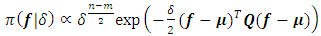(3)

where is a semi-definite matrix of constants with rank . The properties of a particular GMRF are all reflected through matrix . For instance, the Markov properties of GMRFs totally depend on the various sparse structures that the matrix may have. In this paper we use two kinds of GMRFs: second order random walk (RW2) models [16] for metric covariates and intrinsic conditional autoregressive (ICAR) models [17] for spatial covariates. These two GMRFs share equation 3 but with different structures of .

For metric covariates, let be the set of continuous locations and be the function evaluations at , for . Then construction of RW2 model is based on a discretely observed continuous time process that is a realization of an fold integrated Wiener process given by

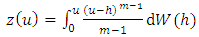(4)

where is a standard Wiener process.

For spatial covariates, letting denote the number of neighbours of site , we assume the following spatial smoothness prior for the function evaluations

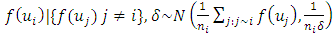(5)

where denotes that site and are neighbors. Thus the conditional mean of is an un-weighted average of evaluations of neighbouring sites.

For the fixed effect parameters , we shall assume independent diffuse priors constant or a weakly informative Gaussian with small precision on the identity matrix . If is a high-dimensional vector, one may consider using Bayesian regularization priors developed in [19], where conditionally Gaussian priors are assigned with suitable hyper prior assumptions on the variances inducing the desired shrinkage and sparseness on coefficient estimates.

2.3. Posterior Inference

The well-known method for estimating Bayesian posterior marginal distribution is Markov Chain and Monte Carlo (MCMC). The alternative method is Integrated Nested Laplace Approximations (INLA) [24]. In this study, INLA method was used because it is generally faster and the solution converges quickly than MCMC for quantile models [20, 24].

2.4. Data Sources

For applications of the methodology, we considered the 2013 Namibia Demographic and Health Survey (NDHS) data. A multistage clustered sampling technique was used to interview a representative sample of more than 2900 eligible women of reproductive age between 15 and 49 years. The anthropometric assessment of themselves and their children that were born within the previous 5 years preceding the survey date was administered. The data set contains information on family planning, maternal and child health, child survival, HIV/AIDS, educational attainment, and other household composition and characteristics.

The primary outcome in this study was the severe childhood (under 5 years) stunting in Namibia. It was assessed by using the adjusted childhood height for age Z-score (HAZ) as a continuous response variable with which corresponded to a HAZ < –3 (the cut-point for severe childhood stunting according to WHO standards). The following bio-demographic and socioeconomic covariates of childhood overweight were assessed in this study: Categorical covariates included sex of household head, type of residence, mother’s education, current mother working status, vitamin A supplementation, vaccination coverage, source of drinking water, type of toilet facility, child HIV status, exclusive breastfeeding, presence of diarrhoea, and household wealth index. Metric covariates included child’s age in months, mother’s body mass index, and duration of breastfeeding in months. The only spatial covariate was regions of Namibia.

2.5. Data Analysis

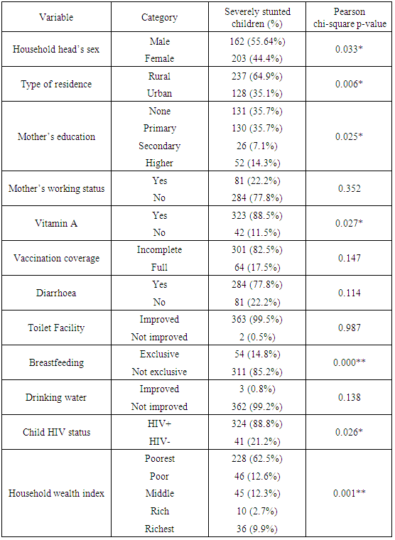
Firstly, we started with exploratory data analysis where basic descriptive analyses such as cross tabulations for all categorical covariates against severe childhood stunting indicator variable were done. The categorized adjusted severe childhood stunting with two categories, severely stunted (HAZ < –3) and not severely stunted (HAZ ≥ –3), was used as a severe childhood stunting indicator variable in this phase. The descriptive statistics (counts, proportions, and chi-square p-values) of all cross tabulations were summarized in Table 1. All covariates of interest were considered in subsequent Bayesian quantile models.

Finally, we fitted various quantile models from which we identified one parsimonious model as the best fitting quantile model using the Deviance Information Criterion (DIC). The DIC is given by where stands for “Deviance evaluated at the posterior mean” and stands for “effective number of parameters”. The rule of thumb is that the smaller DIC values correspond to better model fit. In particular, if model A has smaller DIC (by at least 10 units) than DIC for model B, then model A is more adequate than model B. The statistical inference was fully Bayesian using the INLA approach implemented in R with reference to examples cited in [20].

3. Results

3.1. Exploratory Analysis

Table 1 shows the summary of all cross tabulations of severe childhood stunting by observed categorical covariates. The sex of household head, type of residence, mother’s education, vitamin A supplementation, vaccination coverage, source of drinking water, child HIV status, exclusive breastfeeding, presence of diarrhoea, and household wealth index were all observed significantly associated with severe childhood stunting at 5% level. We observed that severely stunted were the children with male household head, rural residence, less educated mother, no vitamin A supplementation, inadequate vaccination coverage, poor source of drinking water, positive HIV status, non-exclusive breastfeeding, frequent exposure to diarrhoea, and poorer household wealth index.

Table 1. Childhood categorical covariates

3.2. Bayesian Additive Quantile Modelling

All covariates of interest were considered in subsequent in-depth models. Several different Bayesian additive quantile models were fitted and their DICs were used to determine the best fitting model at 18^th quantile level.

3.2.1. Model Selection

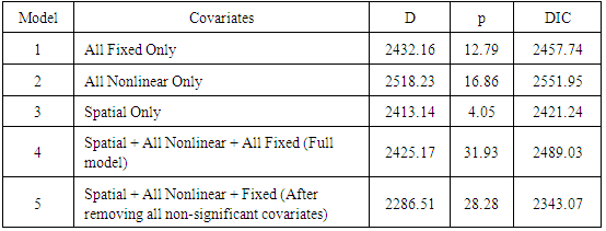
Table 2 displays the summary of DICs for all the models that were fitted. Comparing the DICs in the Table 2, it was observed that model with only structured random spatial effects (model 3) showed a smaller DIC (2421.24) than all models without spatial effects (models 1 and 2) which revealed that the final best fitting quantile model should include the structured random spatial effects. Finally, we observed that model 5 showed smallest DIC value (2343.07) with all fitted covariates being significant. We, therefore, considered it to be the best fitting spatial quantile regression model for severe childhood stunting in Namibia.

Table 2. Comparing DICs for Bayesian regression models

Using the best fitting model 5, we analysed and assessed the fixed effects, nonlinear effects, and structured spatial effects as follows.

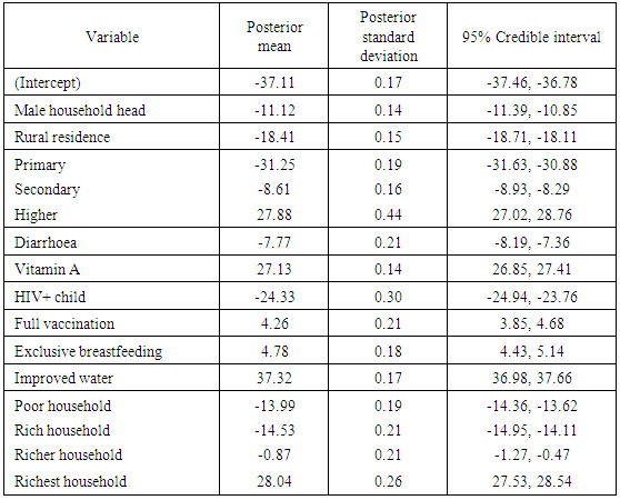
3.2.2. Fixed Effects

A summary of fixed effects on adjusted childhood height for age is shown in Table 3. Male household head showed significant negative effect on adjusted childhood height for age. In other words, severe childhood stunting was more attributable to children belonging to male headed households than those belonging to female headed households in Namibia. This observation was considered significant at 95% credible intervals simply because the interval for male household head was (-11.39, -10.85) which did not include zero. The rest of the table was interpreted in the same way.

In summary, considering 95% credible intervals, we found that the fixed effects of male household head, rural residence, less educated mother, diarrhoea, HIV+ child, and lower household wealth had significant negative relationship with adjusted childhood height for age (i.e. significant positive relationship with severe childhood stunting) whereas more educated mother, vitamin A supplementation, adequate vaccination coverage, exclusive breastfeeding, improved source of drinking water, and highest household wealth had significant positive relationship with adjusted childhood height for age (i.e. significant negative relationship with severe childhood stunting) in Namibia.

Table 3. Fixed effects on adjusted childhood height for age

3.2.3. Nonlinear Effects

Figure 1 shows the summary of observed nonlinear effects. Top plot shows the effects of child age on adjusted childhood height for age while bottom plot shows the effects of duration of breastfeeding on adjusted childhood height for age.

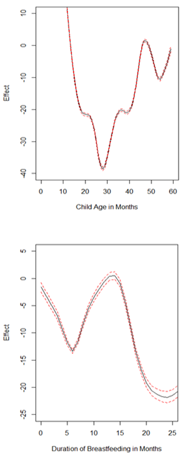Figure 1. Nonlinear effects on adjusted childhood height for age: age of child (top); duration of breastfeeding (bottom)

In general, we found that the nonlinear effects of child age on adjusted childhood height for age generally followed a U-shape relationship. We observed that adjusted childhood height for age rapidly decreases for the first 28 months and thereafter steadily increases. In particular, the adjusted childhood height for age is critically lower for children with ages between 18 and 36 months.

We observed that the nonlinear effects of duration of breastfeeding on adjusted childhood height for age also generally followed an inverse U-shape relationship. In particular, the adjusted childhood height for age is critically lower for children with too short breastfeeding durations (less than 12 months) and longer breastfeeding durations (more than 18 months).

3.2.4. Structured Spatial Effects

Figure 2 presents the posterior means of structured spatial effects on adjusted childhood height for age and their significance at 95% nominal level. Top map shows the distribution of posterior means for structured spatial effects on adjusted childhood height for age. The colours ranged from light green to dark red such that extreme light green and extreme dark red colours respectively corresponded to extreme positive and extreme negative structured spatial effects on adjusted childhood height for age.

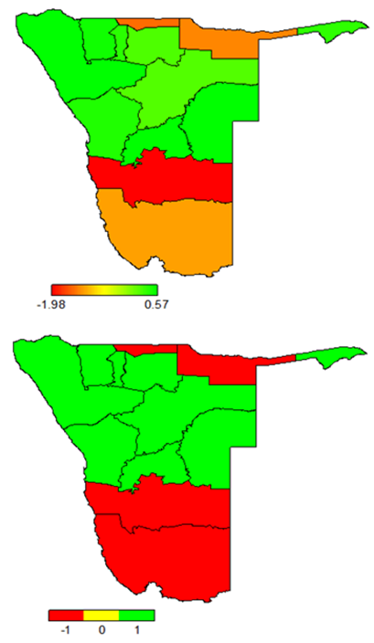Figure 2. Structured spatial effects on adjusted childhood height for age: posterior means (top); significance at 95% nominal level (bottom)

Bottom map displays the distribution of significant observed structured spatial effects on adjusted childhood height for age. Only three colours were used for discriminating significance of the observed effects. Firstly, green colour (1) corresponded to significant positive structured spatial effects on adjusted childhood height for age. Secondly, red colour (-1) corresponded to significant negative structured spatial effects on adjusted childhood height for age. Lastly, yellow colour (0) corresponded to non-significant structured spatial effects on adjusted childhood height for age.

We observed that only Ohangwena, Kavango, Hardap, and Karas regions depicted significant negative structured spatial effects on adjusted childhood height for age (significant positive structured spatial effects on severe childhood stunting) at 95% nominal level. The rest of the regions depicted significant positive spatial effects on adjusted childhood height for age (significant negative structured spatial effects on severe childhood stunting) at 95% nominal level.

4. Discussion

In this study, the fully Bayesian structured additive quantile regression models were fitted for childhood overweight using R-INLA. The primary aim of this study was to fit a spatial quantile regression model which is more appropriate than mean regression model when modelling nutritional status. Only severe childhood stunting was assessed because it is currently the most prevalent undernutrition status among children under-five in Namibia.

The inference used in this study was fully Bayesian. The posterior marginal distributions were estimated using R-INLA package in R 3.1.1. The INLA approach was chosen because it is generally faster than MCMC approach for quantile models [20, 24].

This study actually revealed statistically significant associations between a couple of factors that were considered and severe childhood stunting in Namibia.

Firstly, severely stunted children in Namibia are those belonging to male headed households, residing in rural areas, whose mothers are lowly educated, frequently suffering from diarrhoea, with HIV+ status, inadequate vitamin A supplementation, inadequate vaccination coverage, not exclusively breastfed, belonging to households with poor sources of drinking water, and belonging to households with lower wealth indexes. In particular, severely stunted children in Namibia are those whose mothers’ highest education level is secondary school or lower. Furthermore, we noted a sharp increase in severely stunted children from a minimum of 2.7% among rich households to 9.9% surge among the richest families. A similar trend was observed with a minimum of 7.1% stunted children among mothers with secondary education to a sharp increase to 14.3% for mothers with higher education. It is interesting that extreme riches and extended education of mothers seem to have significant effects on severe childhood stunting. This reveals that despite Namibia being rated as an upper income country, severe childhood stunting is still a problem in the country.

Secondly, severe childhood stunting in Namibia significantly varies with age in a U-shaped nonlinear manner. In general, severe childhood stunting in Namibia rapidly increases for the first 28 months and thereafter steadily decreases up to 59 months. In particular, severe childhood stunting in Namibia is critically higher for children with ages between 18 and 36 months.

Thirdly, severe childhood stunting in Namibia significantly varies with duration of breastfeeding in an inverse U-shaped nonlinear manner. In particular, severe childhood stunting in Namibia is critically higher for children with too short breastfeeding durations (less than 12 months) and longer breastfeeding durations (more than 18 months).

Lastly, severely stunted children in Namibia are those residing in the north especially Ohangwena and Kavango regions and as well in the south especially Hardap and Karas regions.

It is worthy to note that no any in-depth analyses of childhood stunting in Namibia have ever been reported. However, similar studies have ever been done in other countries within sub-Sahara Africa and our key findings in this study were very similar to key findings in such studies like [8, 9].

What we see as the most significant strength of this study is that we effectively managed to identify one best fitting spatial quantile model for severe childhood stunting in Namibia at 18^th quantile level. Furthermore, we modelled severe childhood stunting using the quantile regression approach which is more appropriate than mean regression [10, 12, 19, 25-30]. One significant evident weakness of mean regression is that it explains the relationship between the covariates and average response which is helpless with nutritional responses. Quantile regression was more helpful because it appropriately captured the effects of the observed covariates on severe childhood stunting at 18^th quantile level. If mean regression was used, the consequence would have been modelling average adjusted childhood height for age which would indeed be helpless. If we were interested in moderate childhood stunting, we would capture effects of covariates on childhood stunting at 26^th quantile level by flexibly fixing the tau parameter at which corresponded to a HAZ = –2 (the cut-point for moderate childhood stunting according to WHO standards) [7].

5. Conclusions

Using the best fitting fully Bayesian additive quantile regression model with structured spatial effects at 18^th quantile level, we concluded as follows.

The fixed effects of male household head, rural residence, less educated mother, diarrhoea, HIV+ child, and lower household wealth had significant negative relationship with adjusted childhood height for age (i.e. significant positive relationship with severe childhood stunting) whereas more educated mother, vitamin A supplementation, adequate vaccination coverage, exclusive breastfeeding, improved source of drinking water, and highest household wealth had significant positive relationship with adjusted childhood height for age (i.e. significant negative relationship with severe childhood stunting) in Namibia.

In general, we found that the nonlinear effects of child age on adjusted childhood height for age generally followed a U-shape relationship with critically lower adjusted childhood height for age for children with ages between 18 and 36 months. We also observed that the nonlinear effects of duration of breastfeeding on adjusted childhood height for age also generally followed an inverse U-shape relationship with critically lower adjusted childhood height for age for children with too short breastfeeding durations (less than 12 months) and longer breastfeeding durations (more than 18 months).

We noted a sharp increase in severely stunted children from a minimum of 2.7% among rich households to 9.9% surge among the richest families. A similar trend was observed with a minimum of 7.1% stunted children among mothers with secondary education to a sharp increase to 14.3% for mothers with higher education. It is interesting that extreme riches and extended education of mothers seem to have significant effects on severe childhood stunting. This reveals that despite Namibia being rated as an upper income country, childhood stunting is still a problem in the country.

Furthermore, it was observed that only Ohangwena, Kavango, Hardap, and Karas regions depicted significant negative structured spatial effects on adjusted childhood height for age (significant positive structured spatial effects on severe childhood stunting) at 95% nominal level. The rest of the regions depicted significant positive spatial effects on adjusted childhood height for age (significant negative structured spatial effects on severe childhood stunting) at 95% nominal level.

We recommend that childhood malnutrition policy makers should consider timely interventions based on important socio-demographic factors, child age, maternal factors including duration of breastfeeding, and spatial variation of childhood stunting in Namibia. We further recommend that maternity leave be extended to six months to allow optimal breastfeeding especially to mothers with busy work schedule.

Abbreviations

AIDS: Acquired immunodeficiency syndrome; ALD: asymmetric Laplace density; DIC: Deviance information criterion; GMRF: Gaussian Markov random field; HAZ: Height for age Z-score; HIV: Human immunodeficiency virus; ICAR: Intrinsic conditional autoregressive; INLA: Integrated nested Laplace approximations; MCMC: Markov chain and Monte Carlo; MDG: Millennium development goal; NDHS: Namibia demographic and health survey; RW2: Random walk order 2; UNICEF: United nations children’s fund (formerly United nations international children’s emergency fund); WFP: World food programme; WHO: World health organisation.

ACKNOWLEDGEMENTS

Firstly, we acknowledge the permission granted by Measure DHS to use the 2013 Namibia DHS data. Lastly, we would like to thank all anonymous peer reviewers for their careful scrutiny of the original manuscript.