-
Paper Information
- Previous Paper
- Paper Submission
-
Journal Information
- About This Journal
- Editorial Board
- Current Issue
- Archive
- Author Guidelines
- Contact Us
International Journal of Statistics and Applications
p-ISSN: 2168-5193 e-ISSN: 2168-5215
2016; 6(2): 58-80
doi:10.5923/j.statistics.20160602.05

Graphical Representation of the Power Rates for the Winsorized Modified Alexander-Govern Test
 Abstract
 Reference
 Full-Text PDF
 Full-text HTML
Tobi Kingsley Ochuko , Suhaida Abdullah , Zakiyah Zain , Sharipah Syed Soaad Yahaya
College of Arts and Sciences, School of Quantitative Sciences, Universiti Utara Malaysia, Kedah, Malaysia
Correspondence to: Tobi Kingsley Ochuko , College of Arts and Sciences, School of Quantitative Sciences, Universiti Utara Malaysia, Kedah, Malaysia.
| Email: |  |
Copyright © 2016 Scientific & Academic Publishing. All Rights Reserved.
This work is licensed under the Creative Commons Attribution International License (CC BY).
http://creativecommons.org/licenses/by/4.0/

Aims and Objectives: This research deals with the comparison of the power rates of five different tests, namely: the Alexander-Govern (AG) test, the modified one step M-estimator in the Alexander-Govern (AGMOM) test, the Winsorized modified one step M-estimator in the Alexander-Govern (AGWMOM) test, the t-test and the ANOVA, for two, four and six group conditions, positively and negatively with each of the g- and h- distribution. To see of the five tests which one of them will produce the highest power for g = 0 and h = 0, g = 0 and h = 0.5, g = 0.5 and h = 0 and g = 0.5 and h = 0.5 respectively. Method: A line graph is used to show the graphical representation of the trends of the five listed tests, with respect to the effect size index (d) for two groups and (f) for more than two groups conditions. To see those tests that produced the minimum power value of 0.5 and also those tests that produced a power value of 0.8 and are considered to be sufficient and high. Results: The power values of the five different tests, under normal distribution for two group condition only, shows that the power values of the five tests is above the minimum power value of 0.5. Conclusions: The AGWMOM test produced the highest power values under skewed heavy tailed distribution, for four group condition only, with values of 0.9562 and 0.8336, compared to the other four tests, and the power of the test is regarded as sufficient and high.
Keywords: Power rates, Alexander-Govern (AG) test, the AGMOM test and the AGWMOM test
Cite this paper: Tobi Kingsley Ochuko , Suhaida Abdullah , Zakiyah Zain , Sharipah Syed Soaad Yahaya , Graphical Representation of the Power Rates for the Winsorized Modified Alexander-Govern Test, International Journal of Statistics and Applications, Vol. 6 No. 2, 2016, pp. 58-80. doi: 10.5923/j.statistics.20160602.05.
Article Outline
1. Introduction
- This research centres on the comparison of the power rates of five different tests, namely: the Alexander-Govern test (AG), the modified one step M-estimator (MOM), the Winsorized modified one step M-estimator in the Alexander-Govern test (AGWMOM), the t-test and the ANOVA, with the g- and h- distribution, for two, four and six group conditions respectively. To see of the five tests, which one of them will produce the minimum power value of 0.5 and also, a power value of 0.8 and the test is considered to be sufficient and high.The ANOVA is a classical method of analysis, that have been is applied in different fields of life, such as in medicine, economics, sociology and agriculture, as stated by [24]. Three assumptions have to be fulfilled before the method can work effectively, they are: (i) homogeneity of the variance (ii) normal distribution of the data (iii) independent observations.According to [33] the two major problems confronting the ANOVA, is the appearance of non-normality and variance heterogeneity in a data distribution. As a result, the Type I error rates is increased and the power of the test is reduced. To obtain a good test, Type I error rates should be controlled and likewise the power of the test should not be reduced. This implies that the Type I error rates should not be increased and there should be no loss in the power of the test. The ANOVA is used for comparing the differences between three or more means. It is used for testing the equality of the measure of the central tendency of a data distribution, and is robust to small deviations from normality mainly when the sample size is large enough to guarantee normality, as explained by [29, 30].The ANOVA is very sensitive to the assumption of homogeneity of variance, such that when there is a violation, the result of the analysis could be unreliable: then the p-value becomes too conservative or may be large. Therefore, it is very important to test for the homogeneity of the variance and to check for the equality of the variance assumptions by using the correct test, so as to increase the authenticity of the results [5, 31].The problem of variance heterogeneity has been addressed by few scholars and some alternatives were proposed. [27] Proposed the Welch test that is used for testing the hypothesis of two populations with equal means. It was discussed in different literatures as an alternative to the ANOVA [4, 12, 16, 31]. The Welch test gives a good control of Type I error rates for unequal variances. It is an alternative to the parametric method that deals with heteroscedasticity. However, when the sample size is small and as the group sizes increases, the Welch test fails to give a good control of Type I error rates [28]. [10] Proposed a better alternative to the ANOVA, namely the James test. The James test is used for weighing sample means, as mentioned by different scholars [16, 22, 28]. The James test fails to give a good control of Type I error rates for a small sample size and when the data distribution is non-normal. Both the Welch test and the James test are used for analysing a data distribution that is non-normal with variance heterogeneity [6, 13, 14, 30].The [3] introduced the Alexander-Govern test as a better alternative to the Welch test, the James test and the ANOVA, due to its simplicity in calculation as discussed by [26]. The usage of the robust test statistic such as the Alexander-Govern test is very helpful when the assumption of homogeneity of variance is violated. However, this test has its disadvantages. [26, 17, 20] observed that this method is only effective for a normal data and is not suitable for a non-normal data. Their results showed that the Type I error rates became out-of-control, when the data distribution was not normal. The main reason why it cannot work effectively for a non-normal data is because it uses common mean as its measure of central tendency. Common mean is a highly sensitive measure with 0% breakdown point, even when only one data value is changed the value of the mean will be totally changed. Therefore, this measurement cannot handle any occurrence of outliers as well as a slight deviation from a normal distribution. In finding a solution to this problem, [17] suggested using robust estimator such as the trimmed mean, in different statistical tests that originally used the mean as the central measure of tendency. Their findings proved that by substituting robust estimator such as the trimmed mean to the common mean is able to improve the performance of the tests in terms of Type I error rates, for a non-normal data. Trimmed mean was also used in Alexander-Govern test by [15, 18] and they observed that with the use of Winsorized variance and trimmed mean is able to eliminate the appearance of outliers in a skewed data distribution. This shows that with the use of trimmed mean, non-normality problem can be eliminated. Trimmed mean serves as an estimator that as a substitute for the common mean as a central tendency measure in a data distribution. Trimmed mean have been used by different scholars, due to its efficiency and reliability in putting under control Type I error rates [11, 19, 18]. In applying trimmed mean in a data distribution, it possesses some drawbacks, namely: (i) the percentage of trimming is placed at prior, resulting in the elimination process. (ii) in trimming process, it must be done carefully, to minimize loss of information (iii) it cannot handle large size of extreme value [32]. According to [1] an alternative to the use of trimmed mean in Alexander-Govern test is a highly robust estimator, known as the MOM. It was discovered that when the data distribution is skewed, the MOM estimator gave a good control of Type I error rates. The MOM estimator empirically trims extreme data depending on the nature of the distribution, be it skewed or normal distribution. When it was applied in Alexander-Govern test, it gave a remarkable control of Type I error rates, for a normal or highly skewed data distribution, but it failed to give a good control of Type I error rates under extreme condition of skewness and kurtosis [23].In this research, the Winsorized MOM estimator was applied in Alexander-Govern test to overcome its weakness for non-normality, under variance heterogeneity, in an extreme condition of skewness and kurtosis, to give a remarkable control of Type I error rates and to produce high power for the test.
2. The Alexander-Govern Test and Its Test Statistic
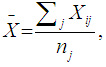
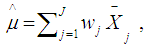
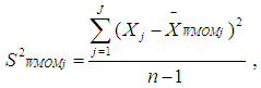
- The Alexander-Govern test was introduced by [3]. This test is used for comparing three or more groups. The mean serves as a measure of the central tendency for the test and gives a good control of Type I error rates for a normal data under variance heterogeneity. But this test is not robust to non-normal data. The test statistic for the test is defined by using the following methods.First, the data sets are ordered, with population sizes of j (j = 1, …, J). For each of the data sets, the mean is calculated by using:
 | (1) |
 is the observed ordered random sample with
  as the sample size of the observations. The mean is used as the central tendency measure in the [3]. After obtaining the mean, the usual unbiased estimate of the variance is obtained by using the formula:
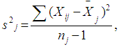 | (2) |
 is used for estimating
  for the population j. The standard error rate of the mean is calculated using the formula below:
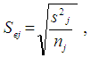 | (3) |
 for the group sizes with population j of the observed ordered random sample is defined, such that
  must be equal to 1. Then the weight
  for each of the groups is calculated using the formula:
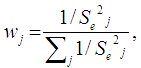 | (4) |
 | (5) |
 , is the weight for each of the independent groups in the data distribution and
  is the mean of each of the independent groups in the observed ordered data sets. The t statistic for each of the independent groups is calculated by using:
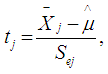 | (6) |
 is the mean for each of the independent group,
  is the grand mean for all the independent groups with population j, the t statistic with nj – 1 degree of freedom. Where
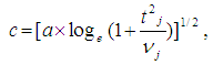
  is the degree of freedom for each of the independent groups in the observed ordered data sets. The t statistic calculated for each of the groups is converted to standard normal deviates by using the [9] normalization approximation in the [3] approach.
 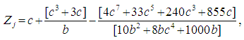 | (7) |
 | (8) |
 | (9) |
 | (10) |
 chi-square degree of freedom is chosen. If the p-value obtained for the AG test is > 0.05, the test is regarded as not significant, otherwise the test is said to be significant.
3. The Winsorized Modified Alexander-Govern Test
- Let the observed ordered data sets of
 with sample
  and group sizes j. Firstly, the median of the data set is calculated by selecting the middle value from the observations. The MAD estimator is the median of the set of the absolute values of the differences between each of the score and the median. It is the median of
  . Therefore, the median absolute deviation about the median
  estimator is calculated using the formula:
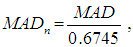 | (11) |
 estimator with the aim of making the denominator estimates
  when sampling from a normal distribution. Outliers in a data distribution can be detected by using:
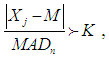 | (12) |
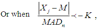 | (13) |
 is the observed ordered random sample,
  is the median of the ordered random samples and
  is the median absolute deviation about the median. The value of
  is 2.24. This value was proposed by [30] for detecting the presence of outliers in a data distribution, because it has a very small standard error, when sampling from a normal distribution. Equation (12) and (13) is also referred to as the MOM estimator that is used for detecting the presence of outliers in a data distribution. In this research, we modified the mean as a measure of the central tendency in Alexander-Govern test, by replacing it with the Winsorized modified one step M-estimator (WMOM) as the central tendency measure for the test. The WMOM estimator is applied on the data distribution, where the outlier value detected is replaced or exchanged with a preceding value closest to the position where the outlier is located. The WMOM estimator is calculated by averaging the Winsorized data distribution. It is expressed as:
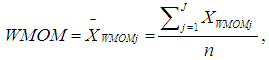 | (14) |
 | (15) |
 is the observed random ordered sample and
  , is the Winsorized MOM estimator for the Winsorized data distribution. The standard error of the WMOM is calculated using the bootstrapping technique. The bootstrapping algorithm for estimating the standard errors is obtained using the following steps.Firstly, we select B independent bootstrap samples expressed as:
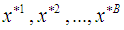 , where each of these random samples consists of
  data values selected with replacement from
  defined as:
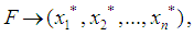
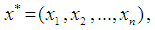 | (16) |
 | (17) |
 shows that
  is not the real data of x, but it refers to a randomized or resampled version of x. In estimating the standard error of the bootstrap samples, the number of B falls within the range of (25 – 200). According to [8] bootstrap sample of size of 50 is sufficient to give a reasonable estimate of the standard error of the MOM estimator. In this research, the same quantity of sample size was used to estimate the standard error of the MOM estimator. Secondly, the bootstrap replications equating to each of the bootstrap samples is defined as:
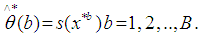 | (18) |
 and
and  is the empirical distribution for the probability of
  on each of the observed values of
  . Thirdly, we estimate the bootstrap estimate of
  from the sample standard deviation of the bootstrap replications that is defined as:
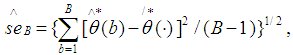 | (19) |
 and
and  .The weight
  for the Winsorized data distribution for each of the independent groups is defined as:
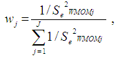 | (20) |
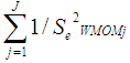 is the sum of the inverse of the square of the standard error for all the independent groups in the observed ordered random samples. Where
  is the standard error of the Winsorized data distribution and is defined as:
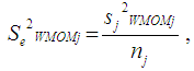 | (21) |
 | (22) |
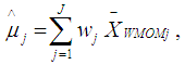
 is expressed as the weight for the Winsorized data distribution and
  is expressed as the mean of the Winsorized data distribution. The t statistic for each of the group is defined as:
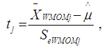 | (23) |
 ,
,  , and
, and  is the Winsorized MOM, the total mean for the Winsorized data distribution and the standard error of the Winsorized data distribution respectively. In the Alexander-Govern technique, the
  value is transformed to standard normal by using the [9] normalization approximation and the hypothesis testing of the Winsorized sample variance of the WMOM estimator for
  is expressed as:
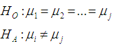 For j = (j = 1, …., J)The normalization approximation formula for the Alexander-Govern technique, using the Winsorized Modified One Step M-estimator is defined as:
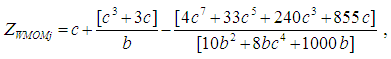 Where
Where 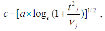
 The test statistic of the Winsorized Modified One Step M-estimator in the Alexander-Govern test for all the groups in the observed random data sample is defined as:
 | (24) |
 level of significance with J – 1 chi-square degree of freedom. The p-value is obtained from the standard chi-square distribution table. If the value of the test statistic for the AGWMOM is < 0.05, the test is considered to be significant. Otherwise the test is regarded as not significant.
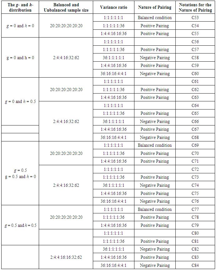
4. Variables Used in This Research
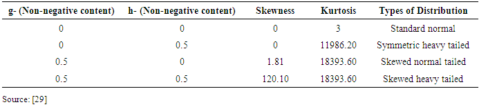
- Five variables were used in this research, namely: balanced and unbalanced sample sizes, equal and unequal variance, group sizes, nature of pairing and types of distribution. All these variables were manipulated to show the strength and weakness of the AG test, the AGMOM test, the AGWMOM test, t-test and the ANOVA respectively.
|
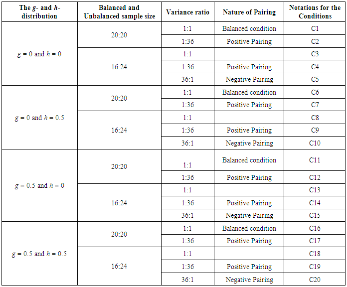
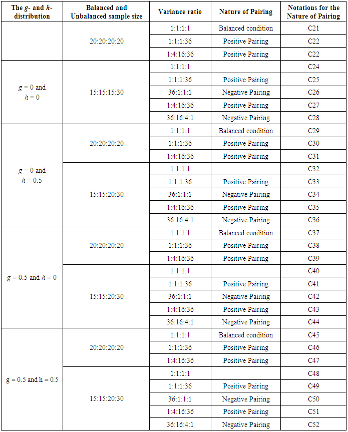
5. The Research Design
- The Alexander-Govern test is a test that uses mean as a measure of its central tendency, but is not robust for non-normal data under variance heterogeneity. For the design of this research, balanced and unbalanced sample sizes were paired with equal and unequal variance for two groups (J = 2), four groups (J = 4) and for six groups (J = 6), positively and negatively with each of the g- and h- distribution.For each of the tests namely: the AG test, the AGMOM test, the AGWMOM test, the t-test and the ANOVA, 5,000 data sets were simulated as a reasonable amount to give good results for the power rates of the five tests respectively. To obtain the pseudo random variates, SAS generator RANNOR [25] was used with a nominal level of α = 0.05 for the analysis of the tests in this research.
|
|
|
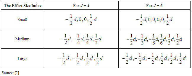
6. The Statistical Power of a Test
- The statistical power of a test is defined as the probability that it will definitely result in significant outcomes [7]. It could also be described as the capacity of a test to recognize any effect when the effect size occurs. [7] Explains that the effect size is the extent at which a phenomenon is observed in the population. As a result, the null hypothesis becomes false in the population. When making hypothesis testing, the probability of accepting the null hypothesis when it is false is known as Type II error, which is denoted by as
 . In addition, the power of a test could be explained as the probability of not accepting the null hypothesis when it is false, and it is represented as
  . The power of a test is affected by three factors, namely: (i) sample size (ii) level of significance (iii) effect size.The sample size: In detecting the power of a test, the selection of the sample size chosen by the researcher is very important. The selection of the sample size directly affects the power of a test. For a small sample size selected, it will result to a very small amount of the power of the test. When the sample size is large, it will definitely result to a large amount of the power of the test. Hence, the selection of the sample size chosen by the researcher will directly affect the power of the test. The power of a test is directly proportional to the quantity of the sample sizes selected [2].[21] Stated that the power of a test must be above 0.5 and can be considered sufficient when the value is 0.8 and above. When the power of a test is 0.8, it shows that success which is the probability of not accepting the null hypothesis is four times as certain as failure. When the power of a test is 0.9, it shows that the success is nine times as certain as failure.The level of significance: It is the process of neglecting the null hypothesis when it is actually true, and is otherwise referred to as Type I error. The level of significance is expressed as α, and it has a value which is equal to 0.05 [7]. The level of significant chosen in this research is 0.05. Effect Size: In statistics, it is observed that the probability of the null hypothesis, that is p-value, decreases as the effect size increases and the sample size increases accordingly. The effect size could also be defined as the extent a given phenomenon is observed in the population, resulting to a state whereby the null hypothesis is false in that population. The effect size shows the differences between the maximum and minimum means between two groups, divided by the standard deviation inside the population [7].Large pattern of variability was chosen in this research for each of the tests, namely the AG test, the AGMOM test, the AGWMOM test, the t-test and the ANOVA, in order to obtain high power for the tests.
|
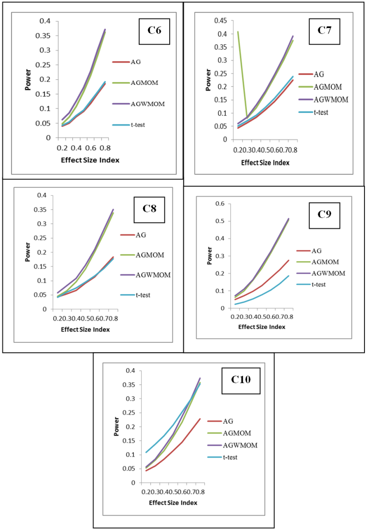
7. The Power Rates of the Tests
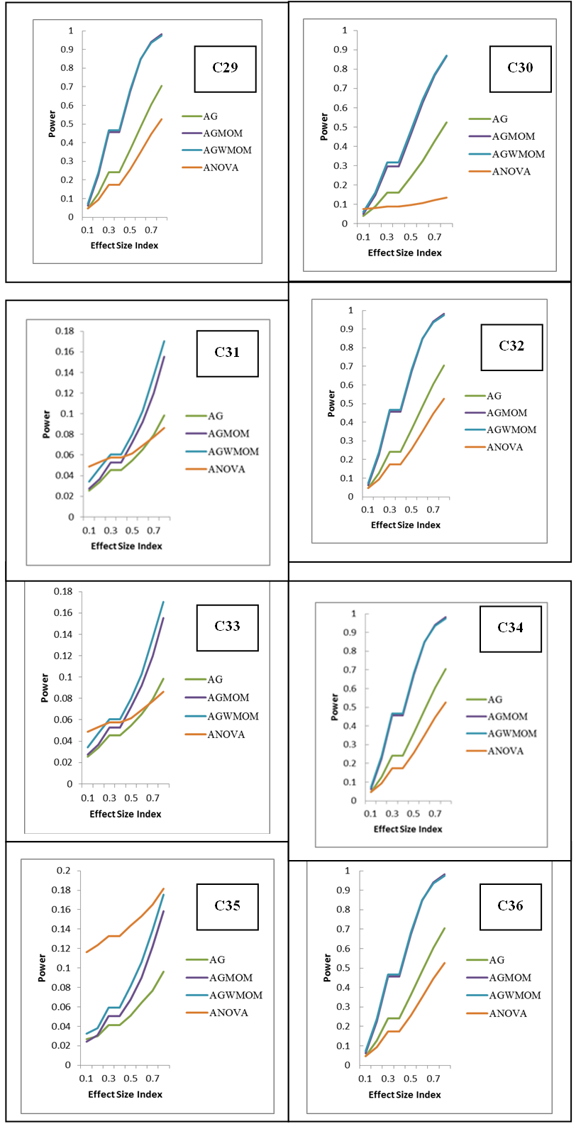
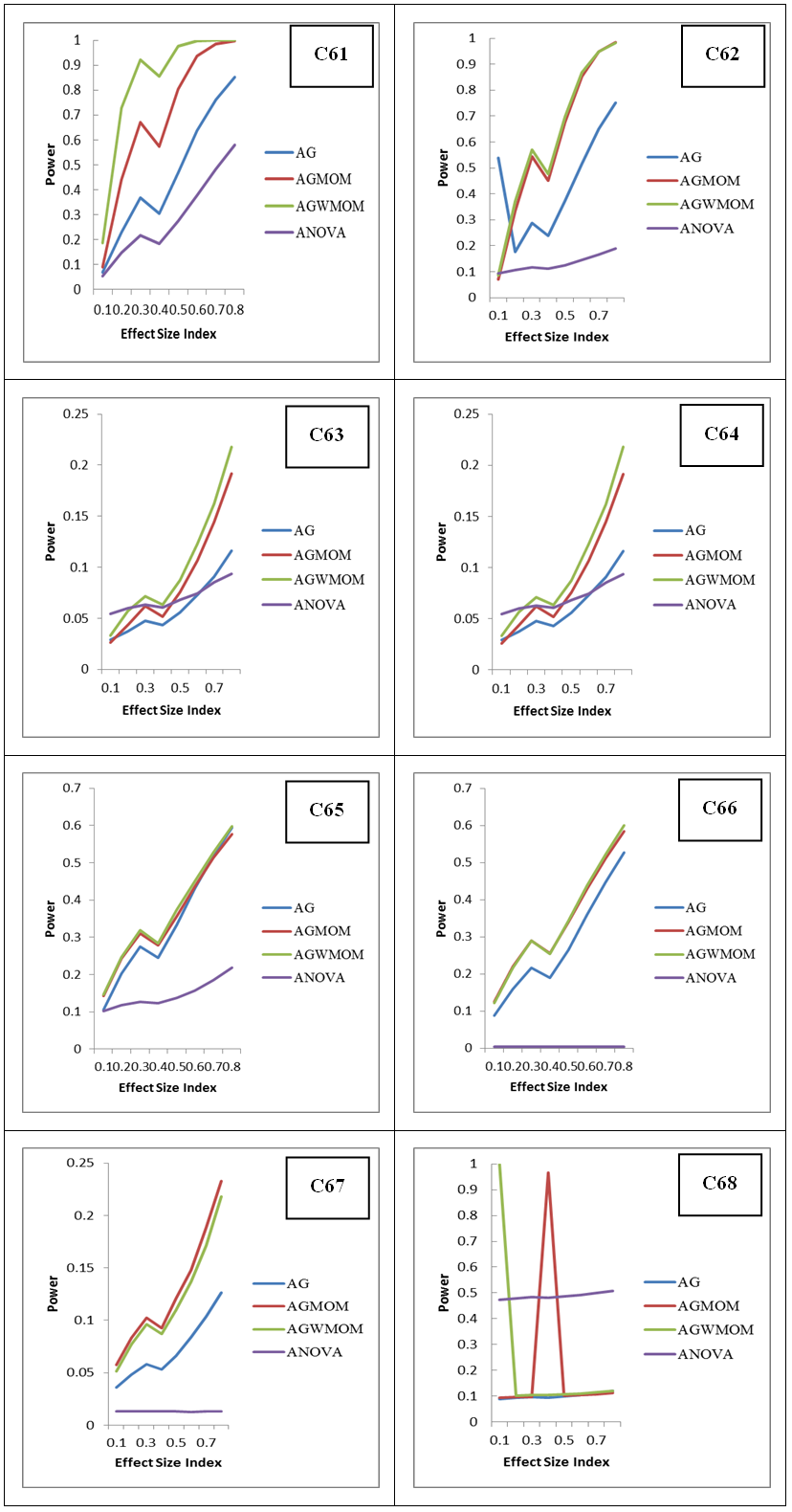
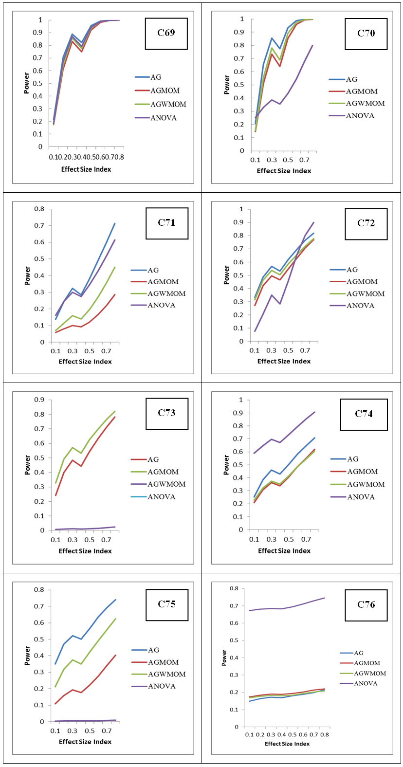
- The power rates of the tests is represented graphically, where the y-axis corresponds to the power of the tests and the horizontal axis represents the effect size index d for two groups case and f for more than two group case. The graph is used to show the trend of the power of the tests in relation to the effect size index. According to [21] the power of a test must be above 0.5. It can be considered sufficient and high when its value is 0.8 and above.The graph shows those tests that have low power, sufficient and high power with respect to the effect size indexes (d and f). In this research, the effect size index is used for the analysis of the power rates of the five different tests accordingly.
8. Graphical Representation of the Power Rates of the Tests
 | Figure 1. Power versus Effect Size Index, for Two Group Condition, Under a Normal Distribution |
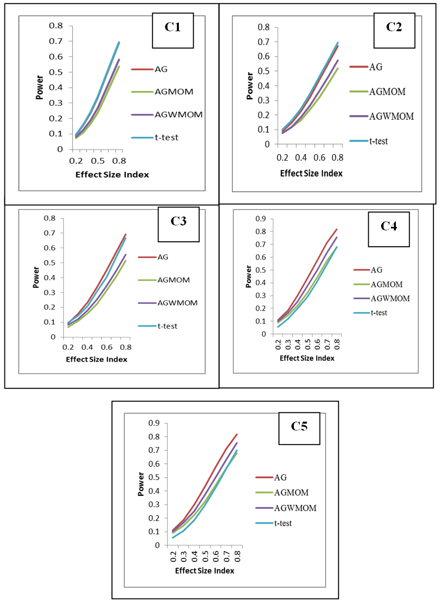 | Figure 2. Power versus Effect Size Index, for a Symmetric Heavy Tailed Distribution, for Two Group Condition |
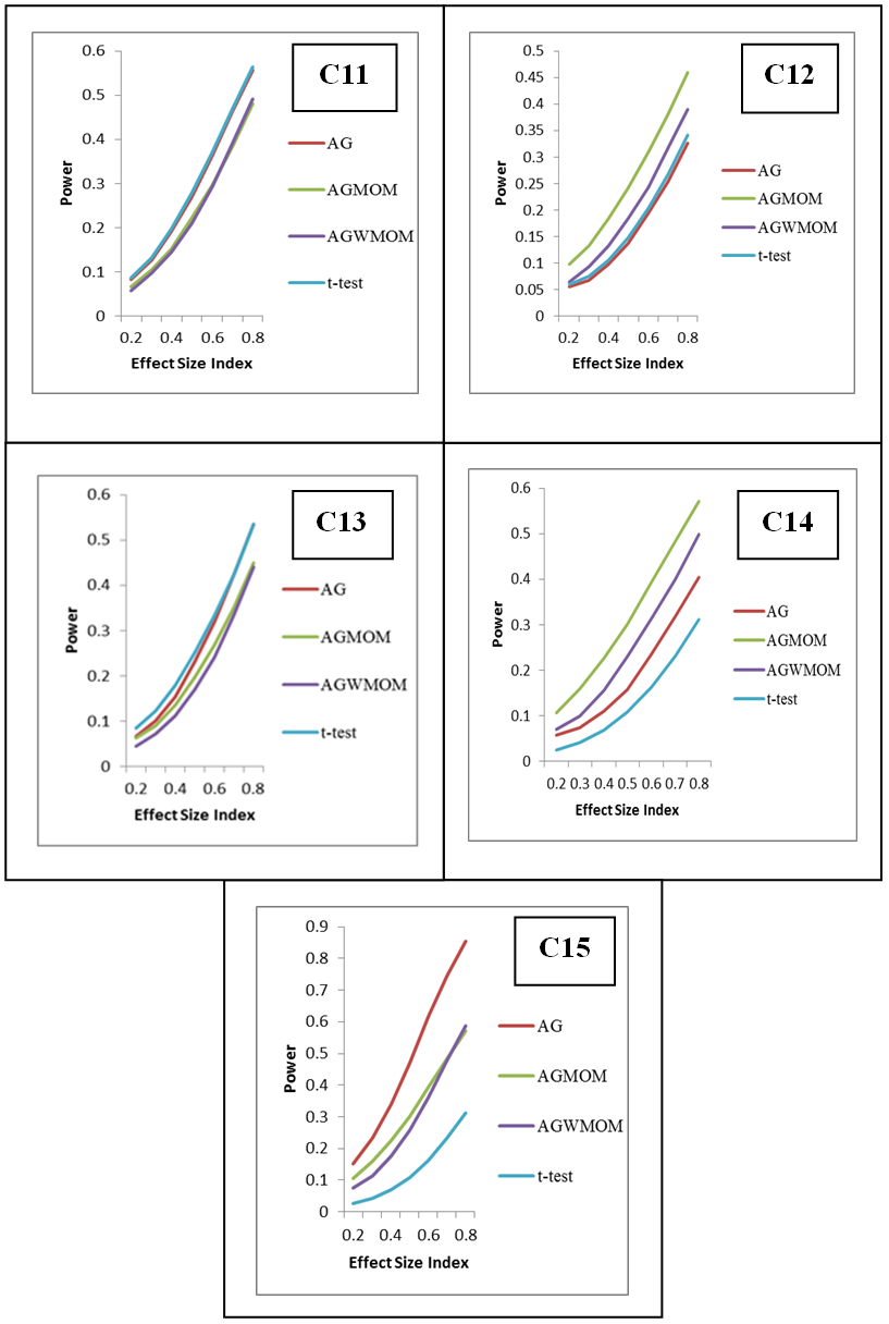 | Figure 3. Power against the Effect Size Index, for Two Group Condition, Under a Skewed Normal Tailed Distribution |
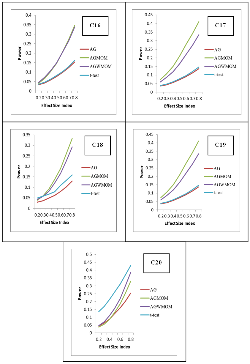 | Figure 4. Power versus Effect Size Index, for Two Groups Condition, Under a Skewed Heavy Tailed Distribution |
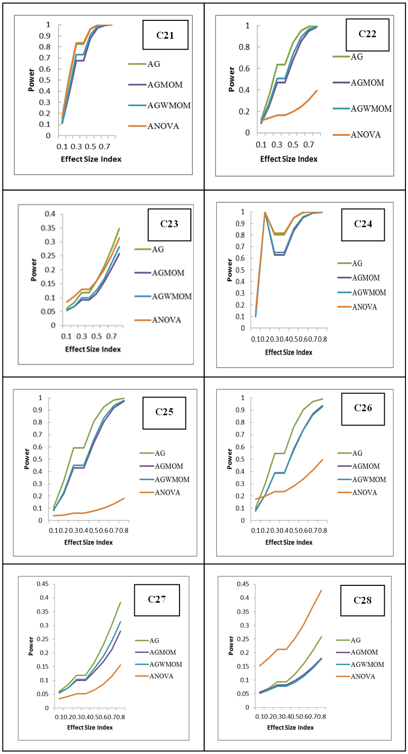 | Figure 5. Power versus Effect Size Index, for Four Groups Condition, Under a Normal Distribution |
 | Figure 6. Power versus Effect Size Index, for Four Group Condition, Under a Symmetric Heavy Tailed Distribution |
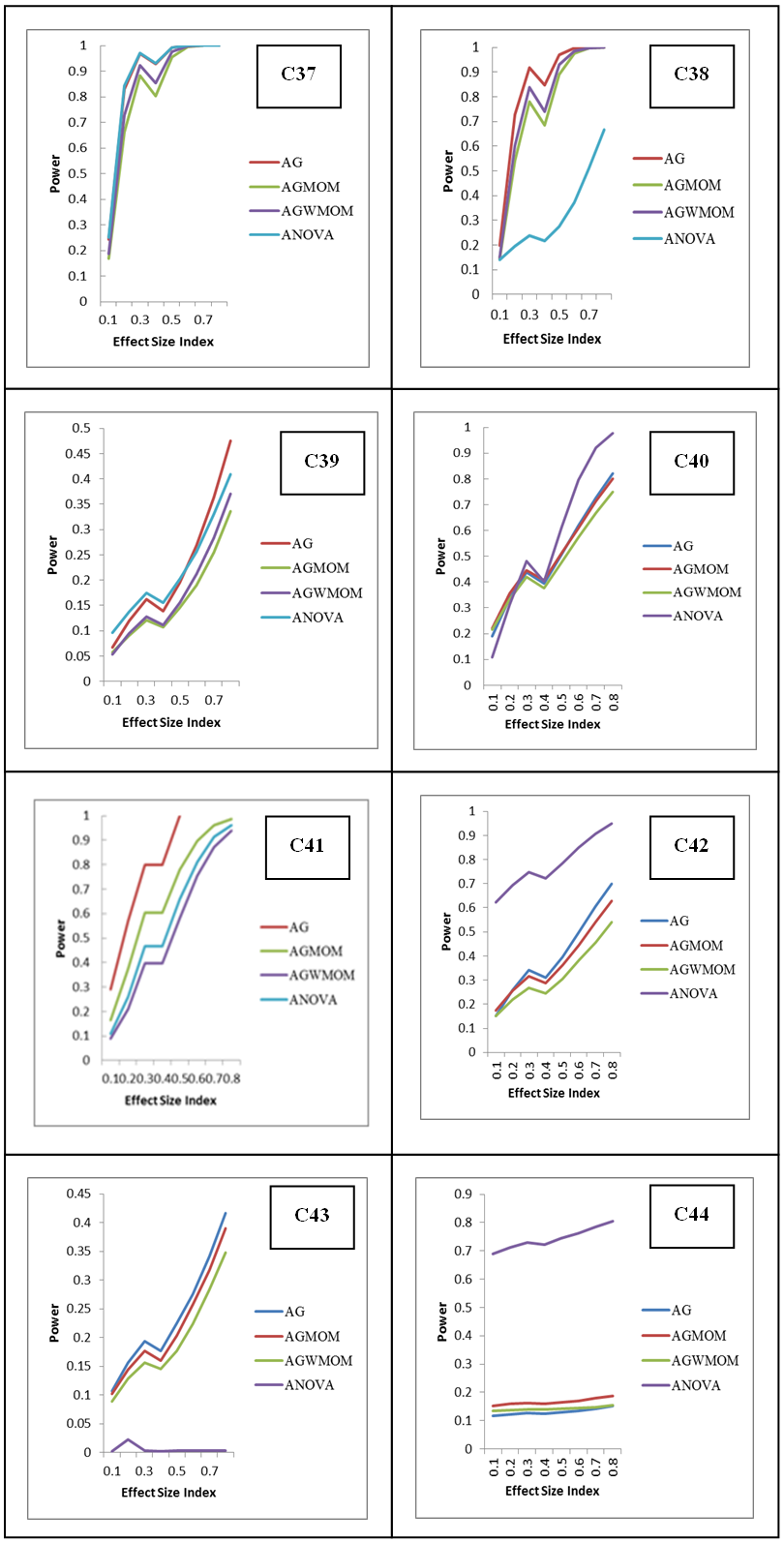 | Figure 7. Power against Effect Size Index, for Four Groups Condition, Under a Skewed Normal Tailed Distribution |
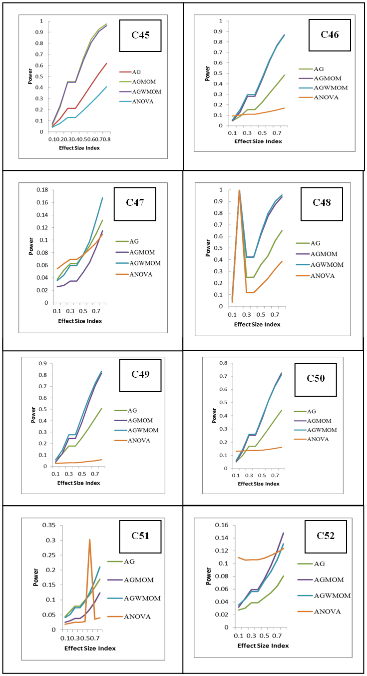 | Figure 8. Power versus Effect Size Index, for Six Groups Condition, Under a Skewed Heavy Tailed Distribution, for Four Groups Condition |
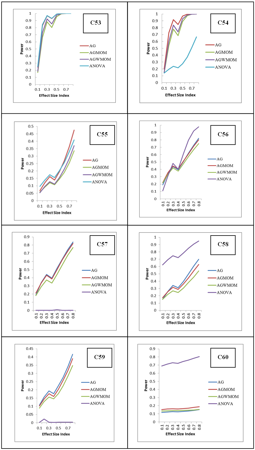 | Figure 9. Power versus Effect Size Index, for Six Groups Condition, Under a Normal Distribution |
 | Figure 10. Power against the Effect Size Index, for Six Groups Condition, Under a Symmetric Heavy Tailed Distribution |
 | Figure 11. Power versus Effect Size Index, for Six Groups Condition, Under a Skewed Normal Tailed Distribution |
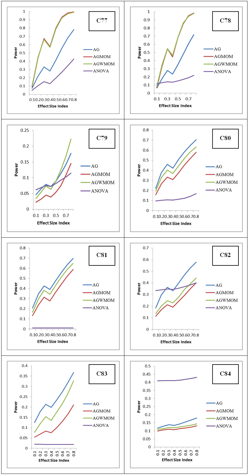 | Figure 12. Power versus Effect Size Index, for Six Groups Condition, Under a Skewed Heavy Tailed Distribution |
9. Conclusions
- According to [21] the power of a test must be 0.5 and above and is referred to as sufficient and high when its power value is 0.8 and above. In this research, the AGWMOM test produced a high power value of 0.9562 with the pairing of unbalanced sample size of (15:15:20:30) with equal variance of (1:1:1:1) and high power value of 0.8336, with the pairing of unbalanced sample size of (15:15:20:30) with unequal variance of (1:1:1:36) under skewed heavy tailed distribution, for four group conditions only, compared to the AG test, the AGMOM test, the t-test and the ANOVA and the power of test is referred to as high and sufficient.
ACKNOWLEDGEMENTS
- I give all the thanks, praises, glory, honor, adoration, power and worship to God Almighty for everything. He is the author of wisdom, knowledge and understanding. The Everlasting Father, “The beginning and ending of everything”.I also want to thank and acknowledge my wonderful, blessed, ever-loving, caring and ever-dynamic parents, in person of Mr. and Mrs. D.K.O. Tobi, for their constant encouragement, love, support, backings, sacrifice and goodwill in the course of carrying out this research. I love and appreciate them very greatly.