1. Introduction

1.1. Propensity Score

Propensity Score Matching (PSM) is the current popular method used to evaluate the impact of the programmes compared to other non-experimental methods [6]. It is used in diverse fields of study [4]. The method is the most widely used type of matching in which the comparison group is matched with the treatment group on the basis of a set of observed characteristics or by using the propensity score (PS) [2]. PS is a predicted probability of participation given observed characteristics or variables [15] & [7]. These variables are selected in such a way that they are not affected by the treatment.

PSM originated from the statistical literature and shows a close link to the experimental context. Its basic idea is to find in a large group of non-participants, those individuals who are similar to the participants in all relevant pre-treatment characteristics X [3]. PS is used to compare the treatment units in the observational studies in order to determine the causal effects when the treatment assignment is not random. In statistics, this comparison is called matching. The statistical matching technique that attempts to estimate the effect of a treatment, policy, or other intervention by accounting for the covariates that predict receiving the treatment is called PSM [1]. The closer the propensity score, the better the match.

Baker [2] argues that matching methods or constructed controls try to pick an ideal comparison that matches the treatment group from a larger survey. The main reason is that, through PSM, the selection bias can be controlled. Rosenbaum and Rubin [13] who are the founders of PSM outline that the bias is removed through observed covariates.

Although PSM has emerged as a most widely used method in measuring non-experimental design, it suffers from debates. One of the major debates of PSM is its functional form. Despite the model specification being one of the areas which needs further research, a few researchers have focused on this area. Following the different arguments about the implementation of PSM in the literature, the paper intended to analyse the effects of the weighted data in generating PS.

1.2. Data Weighting

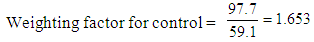
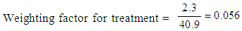
Data weighting plays a major role in an analysis as it produces the estimates of statistics that would have been obtained if the entire sampling frame had been surveyed [9]. Because of this, it is important to weight the data before the analysis. Unweighted data implies that each case counts the same as any other case. Moreover, it is assumed that each case has equal probabilities of being selected and non-coverage and non-response are equal among all units of the population. It is very difficult for the assumptions to be met as during data collection the differences may arise hence this can affect the results. The differences can be caused by the sampling variability, differential under coverage, and possible response errors such as differential response rates or misclassification errors. The weighting for each case can help to adjust the differences.

In this paper, the weighting is considered since the sample was not representative (not proportionally selected) for the targeted population. The targeted population in five regions were 10,686,449 of which 242,000 were participant farmers and 10,444,449 were non-participants farmers. The population proportion of participating farmers was 2.3% (242,000/10,686,449 x 100) while for non-participating farmers was 97.7%. In the sample, the participating farmers accounted for 40.9% (359/878 x 100) while non-participating farmers accounted for 59.1%. The participating farmers sample size was high compared to population size.

Because the sample was disproportional (sample was not representative for population), the weighting was considered in order to adjust the samples composition to be reflected by the population’s composition. The disproportion sample leads to overrepresentation or underrepresentation which actually affects the study result. The study weighted the data in order to correct disproportional sample size. Through data weighting, the sample bias is reduced since underrepresentation or overrepresentation of population makes the sample biased.

The weighting is good when dealing with an aggregate data. Since the interest in PSM is to estimate the average effects, then weighting is preferable. Through weighting, it is expected that, the matching scores are improved. The propensity scores are the expected outcome of the given covariates (pre-treatment characteristics).

Before running PSM, the weighting factors were calculated using the equations 2 and 3. The weighting factors were obtained by taking a ratio of percent in population over percent in sample.

(1)

(2)

(3)

Thereafter, the data were weighted by case using weight for treatment 0.06 and weight for control 1.65.

2. Materials and Methods

The data were collected through the mixed approach as the data collected were both numerical and categorical from five Tanzania regions namely: Kagera, Mwanza, Mara, Simiyu and Kigoma. Within the regions, the focus was an agro-ecological zone where the corn was cultivated. The research design adopted was non-experimental cross-sectional survey. The study was non-experimental due to the fact that the units studied were not randomly assigned. The cross-sectional strategy was adopted as the information was collected at one point of time. On the other hand, it was a survey since large data was collected on a wide range. The data was collected from 878 corn farmers through self-administered delivered and collection questionnaire and interview.

PS was generated using Logistic Regression (LR) model. LR was used because it is the most powerful model compared to others when the response variable is binary [11]. It is more flexible and robust method compared to linear discriminant analysis (LDA) especially when there are violations of assumptions [12]. Thirteen confounding variables involved in PS estimation included: sex, age, type of farmer, marital status, level of education, household size and land owned. Others were, the distance from home to corn farm (km), distance from the village to district headquarters (km), distance to tarmac road (km), weather, soil type and membership of other participatory farmer groups. These variables were believed to be enough as too many variables affect common support as suggested by Heinrich [7]. There were other variables such as land area owned for corn cultivation (ha), mode of farming, etc. that were not included in the model. The variables were excluded in the model because they affected matching balance of univariate and multivariate statistics tests.

The t-test was used to compare PS generated from sample of farmers not participating in agriculture intervention (control) to those participating the intervention (treatment).

3. Results and Discussion

3.1. Result of LR Model

This subsection provides result of contribution of each variable in LR model. Examination of variables in the model was done basing on p-values and odds ratio. Result of LR is presented in Table 1.

Table 1. Result of LR

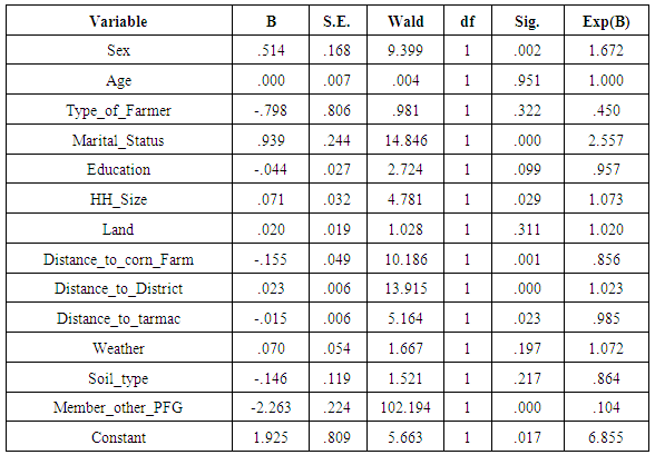
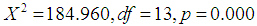LR result shows that, baseline model (confounding variables excluded) was accurate by 56.2%. This indicates that by nature the model has predictive power. Omnibus tests of model coefficients showed further that, chi-square is significant at 0.05. This implies that, the full model (all confounding variables included) is improved. Nagelkerke measure suggests that, the model explains about 28.7% of the variation in the outcome. The Hosmer-Lemeshow statistic indicates a good fit because 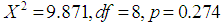. Classification rate accuracy of full model is improved as it stands at 70.9% compared to 56.2% of baseline model.

From Table 1, it can be seen that, out of thirteen variables included in the model, about seven were significant as their p-values were less than 0.05. These are sex (p = 0.002), marital status (p=0.000), household size (p=0.029), distance to corn farm (p=0.001), distance to district (p=0.000), distance to tarmac (p=0.023) and participation in other PFG (p=0.000).

Odds ratio (OR) shows that, seven have odds ratio values greater than or equal to 1 which indicates that, their contribution to the model was positive. The variables are sex (OR =1.672), Age (OR = 1.000), marital status (OR = 2.557), household size (OR = 1.073), land (OR = 1.020), distance to district (OR = 1.023) and weather (OR = 1.072). The remained six variables have less contribution to the model.

The interest of the paper was to generate PS and not statistical contribution of individual variable in the model. Basing on this, generation of PS using weighted and unweighted data included all thirteen variables in the LR model as presented in subsections 3.2 and 3.3. Inclusion of all variables in the model was in line to Domingue and Briggs [6], Carver [5], Morse [10] and Schmidt and Hunter [14] who suggest that, the significance of the variables is of no importance as far as they theoretically relate with the decision of participating or not participating in the programme. Josephat and Ismail [8] suggest that if focus is modelling and not significance of the dimensions, it is proper not to drop any variable as long as they theoretically related to dependent variable.

3.2. PSM Generated from Unweighted Data

Before generating PS, the univariate and multivariate balance statistics tests were analysed and indicated that there were no imbalance after matching. Josephat and Likangaga [8] discuss in detailed on testing the univariate and multivariate balance statistics for unweighted data. The dotplot of standardized mean differences is presented in Figure 1. From the figure, it can be seen that after matching, PS becomes very close to dashed line (matching marks are bolded) compared to unmatched PS. The sex covariate has matched the scores almost in line with the dashed line. Other variables with PS points which lie in a dashed line include: type of farmer, marital status, education, household size and land. The rest of the covariates had PS a bit far from the dashed line. The dotplots of the standardized mean difference show that PS was improved after employing PSM.

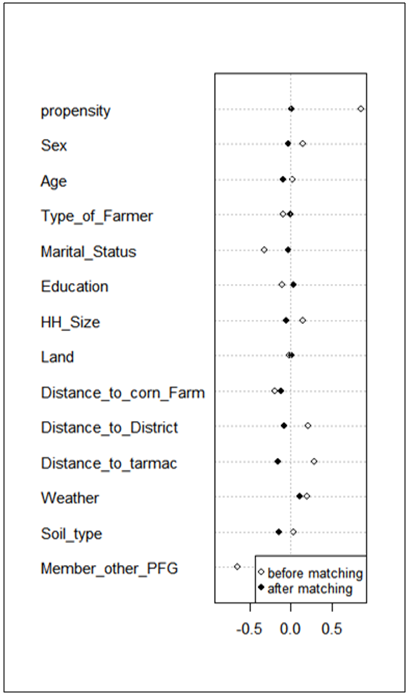Figure 1. Dotplot of Standardized Mean Differences

3.3. PSM Generated from Weighted Data

From a new set of the weighted data, PSM was performed. The results showed that out of 519 control farmers, 231 were matched, 285 were unmatched while 3 were discarded. For the case of the treated farmers, out of 359 farmers, 231 were matched, 128 were unmatched and none was discarded. This result is the same as that obtained when PSM was performed without considering weight (Refer Josephat and Likangaga, 2015).

All univariate and multivariate balance tests showed that there was no imbalance of matches as 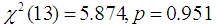was insignificant and for unmatched solution (before matching) was 0.998 while after matching it became 0.996. Furthermore, the standardized mean difference showed that all covariates were balanced as . There is a slight difference in visualization of propensity scores in graphs between those weighted and those not weighted (See Figures 2 and 3). If Figure 2 is compared to Figure 4, it can be observed that there is an improvement of matched PS in Figure 2 as the bolded lines for all data and matched data lie below 0.1.

This shows that there are improved matches of propensity scores between the control and treatment groups since there is less deviation of an absolute standardized difference in mean for the weighted data.

It can further be observed that the propensity scores for variables age, distance to district, distance to tarmac road, weather and soil type lie or became very close to dashed line in Figure 3 than in Figure 1. This indicates that the weighted data provide the improved matching of propensity scores.

To test whether PS generated from the weighted data for control and treatment groups are different, the independent t test was used. The result shows that the correlation coefficient of the propensity scores among the two groups is significant . The mean difference of propensity score of the two groups (0.000636) is insignificant 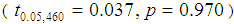. The result indicates that the propensity scores generated are very similar between control and treatment. There is a slight difference of mean (0.000751) between propensity scores of the weighted and unweighted data. The weighted data slightly improves the propensity scores than unweighted data.

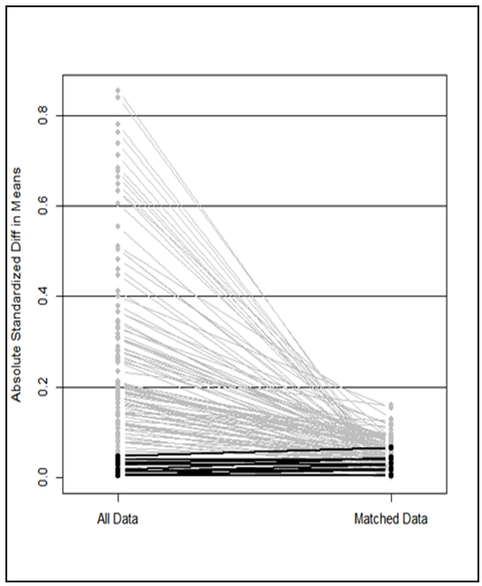Figure 2. Lineplot of Standardized Differences for Weighted Data

Figure 3. Dotplot of Standardized Mean Differences for Weighted Data

Figure 4. Lineplot of Standardized Differences for un-weighted Data

4. Conclusions

Basing on the findings, it can be concluded that the representative sample for the population produces better PS compared to unrepresentative samples. This suggests that it is very important to weight the data when dealing with the aggregate data for case sample which is not representative of the population. The paper provides the knowledge for the new procedure to conduct PSM where by the data should be weighted before including the variable in the model. Weighted data improves results compared to unweighted data. For the better results of the impact of the programme, the logistic regression model with the sample data which is representative of the population should be used.