-
Paper Information
- Next Paper
- Previous Paper
- Paper Submission
-
Journal Information
- About This Journal
- Editorial Board
- Current Issue
- Archive
- Author Guidelines
- Contact Us
International Journal of Statistics and Applications
p-ISSN: 2168-5193 e-ISSN: 2168-5215
2016; 6(2): 45-52
doi:10.5923/j.statistics.20160602.03

Using Real Life Data to Validate the Winsorized Modified Alexander-Govern Test
 Abstract
 Reference
 Full-Text PDF
 Full-text HTML
Tobi Kingsley Ochuko , Suhaida Abdullah , Zakiyah Zain , Sharipah Syed Soaad Yahaya
College of Arts and Sciences, School of Quantitative Sciences, Universiti Utara Malaysia, Kedah, Malaysia
Correspondence to: Tobi Kingsley Ochuko , College of Arts and Sciences, School of Quantitative Sciences, Universiti Utara Malaysia, Kedah, Malaysia.
| Email: |  |
Copyright © 2016 Scientific & Academic Publishing. All Rights Reserved.
This work is licensed under the Creative Commons Attribution International License (CC BY).
http://creativecommons.org/licenses/by/4.0/

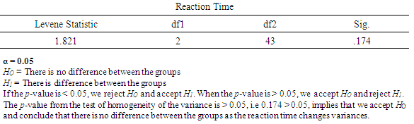
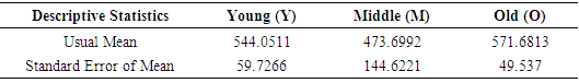
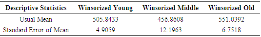
Aims and Objectives: To evaluate the efficiency and reliability of the Alexander-Govern (AG) test and the Winsorized Modified One Step M-estimator in the Alexander-Govern (AGWMOM) test, using real life data. Methods: Test of homogeneity of variance was done from real life data, comprising of young, middle and old groups, using the Levene’s test to see if the three groups are different from each other or not as the reaction time changes. Descriptive statistics, Test of normality and Test Statistic were performed for the three independent groups, to evaluate the reliability and efficiency of the tests. Results: The p-value from the test of homogeneity of the variance is greater than 0.05, i.e 0.174 > 0.05 and it shows that we accept HO and conclude that there is no difference between the groups as the reaction time changes. The descriptive statistics show that the AGWMOM test has a smaller standard error compared to the AG test. The result of the test statistic reveals that the AGWMOM test produced a p-value of 0.0000002869 that is considered to be significant compared to the AG test that produced a p-value of 0.0698 that is regarded as not significant, since its p-value is > 0.05. Conclusions: The AGWMOM test is more efficient and reliable in minimizing error as much as possible from the real life data, because the test produced a smaller standard error from the real life data in comparison to the AG test and is regarded as significant.
Keywords: Alexander-Govern (AG) test, AGWMOM test and Test Statistic
Cite this paper: Tobi Kingsley Ochuko , Suhaida Abdullah , Zakiyah Zain , Sharipah Syed Soaad Yahaya , Using Real Life Data to Validate the Winsorized Modified Alexander-Govern Test, International Journal of Statistics and Applications, Vol. 6 No. 2, 2016, pp. 45-52. doi: 10.5923/j.statistics.20160602.03.
Article Outline
1. Introduction
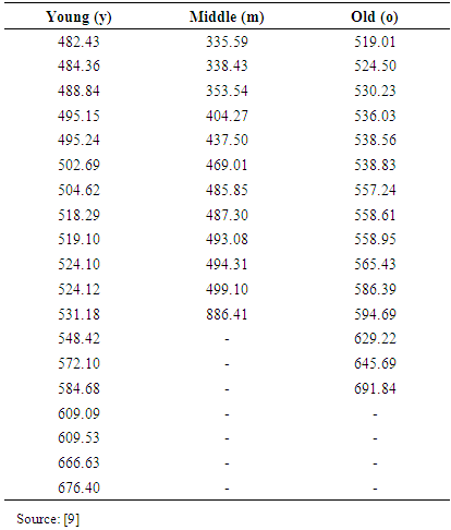
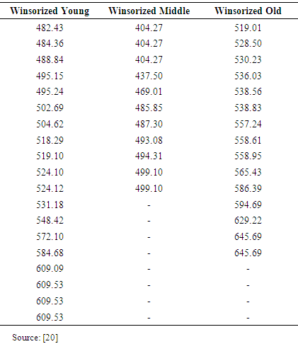
- The independent group tests such as the ANOVA have been employed in different fields of life, such as in economics, sociology, medicine and agriculture as stated by [23]. Some assumptions have to be fulfilled before the method can perform effectively, such as: (1) homogeneity of the variances, (2) normality of the data and (3) independent observations. The ANOVA is classical method of analysis that is used for comparing the differences between three or more means. It is used for testing the equality of the measure of the central tendency and is robust to small deviations from normality, mainly when the sample size is large enough to guarantee normality, as explained by [28, 29].It is observed that the two major problems confronting the ANOVA is the appearance of non-normality and variance heterogeneity in a data distribution [32]. As a result, the Type I error rates are increased and the power of the test is reduced.The ANOVA is very sensitive to the assumption of homogeneity of variance, such that when there is a violation, the result of the analysis could be questionable, since the p-value becomes too conservative. Therefore, it is very important to test for the homogeneity of the variance in order to verify the equality of the variance assumptions by using the correct test, so as to increase the validity of the results [4, 30]. The problem of heterogeneity of variance has been discussed by few scholars and some alternatives have been introduced. [26] Introduced the Welch test that is used for testing the hypothesis of equality of means between two or more populations. It was discussed in different literatures as an alternative to the ANOVA [3, 11, 15, 30].The Welch test gives a good control of Type I error rates for unequal variances. It is a common alternative to parametric methods which deal with unequal variances. However, for a small sample size, the Welch test fails to give a good control of Type I error rates, as the number of groups increases [27]. [8] Introduced a better alternative to the ANOVA, namely the James test. The James test is used for weighing sample means as discussed in different literature by different scholars [15, 21, 27]. For a small sample size and when the data distribution is non-normal, the James test fails to give a good control of Type I error rates. The Welch test and the James test are used for analysing data which are not normally distributed and have unequal variances [5, 12, 13, 29].Alexander-Govern [2] introduced the Alexander-Govern test as a better alternative to the Welch test, the James test and the ANOVA, due to its simplicity in calculation. [24, 16, 19] agreed that the Alexander-Govern test performs well under variance heterogeneity for a normal data, but this test fails to give a good control of Type I error rates for a non-normal data. The reason is because the test uses mean as a measure of its central tendency. The common mean is a very good estimator for a normal distribution, but it is extremely sensitive to the presence of outliers. The common mean cannot handle any slight deviation from normality. In finding a solution to the problem of non-normality, [16] proposed the trimmed mean to handle the problem of non-normality in Alexander- Govern test. Also, [14] and [17] observed that the use of Winsorized variance and trimmed mean is capable of removing the appearance of outliers in a skewed data distribution. This shows that with the use of trimmed means, the non-normality problem can be addressed. Trimmed mean is an estimator which is used in replacing the common mean as a measure of central tendency for a non-normal data. This estimator has been used by different scholars in the past, because of its reliability and efficiency in controlling Type I error rates under non-normality [10, 18, 17]. The application of the trimmed mean in a data distribution has some weaknesses which are: (1) the percentage of trimming-in determining the elimination process must be set in advance. (2) It leads to loss of information, as the data is trimmed symmetrically from both tails of the data distribution. (3). It fails to handle large count of extreme values [31].According to [1] an alternative to the use of trimmed mean in Alexander-Govern test is a highly robust estimator, known as the Modified one-step M-estimator (MOM). It was observed that when the distribution of the data is skewed, the MOM estimator gave a good control of Type I error rates. The MOM estimator empirically trims extreme data set depending on the nature of the distribution, be it skewed or normal. When it was applied in Alexander- Govern test, it gave a remarkable control of Type I error rates under normal or highly skewed data distribution, but this estimator fails to give a good control of Type I error rates, in an extreme condition of skewness and kurtosis [22]. According to [20] Winsorization is the process of making a replacement of an outlier value with the closest (non-outlier) value. Winsorization helps prevent loss of information in a data distribution. The sample size of the data sets is preserved unlike the trimmed mean procedure, where the data is trimmed symmetrically from both tails of the data distribution, resulting in sample size decrease. In this research, the Winsorized Modified One Step M-estimator was applied Alexander-Govern test to overcome the weakness of the MOM estimator in the AG test, in an extreme condition of skewness and kurtosis and to make the test robust to non-normality.The AG test and the AGWMOM test were validated using real life data from [9]. Test of Homogeneity of variances was done for the three independent groups from the real life data, comprising of young, middle and old group and the result show that the three independent groups are not different from each other as the reaction time changes. Test of normality was also performed on the three independent groups, to see which groups are normally distributed. Test statistic were calculated for the two tests, namely the AG test and the AGWMOM test and it showed that the AGWMOM test is more reliable and efficient in minimizing error as much as possible from the real life data, because it produced a p–value of 0.0000002869 compared to the AG test that produced a p-value of 0.0698.
2. The Alexander-Govern Test and Its Test Statistic
- The [2] introduced the Alexander-Govern test. This test uses mean as a measure of its central tendency and it gives a good control of Type I error rates and high power, under variance heterogeneity for a normal data. This test is not robust for non-normal data. This test is used for comparing two or more means and its test statistic is obtained using the following techniques.Firstly, to obtain the test statistic for the Alexander-Govern test, we order the data sets, comprising of J groups indexed by j (j = 1,…,J). Then, for each of the data sets, the mean is obtained by using the formula:
 | (1) |
 represent the observed ordered random observations in samples of size
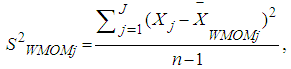
  . The mean is used as a measure of the central tendency in the [2] method. After the mean is obtained, the usual unbiased estimate of the variance is calculated, using the formula:
 | (2) |
 is used to estimate
  for the population j. The standard error of the mean is obtained by using the formula:
 | (3) |
 for the group of the observed ordered random sample is defined, such that
  equal to 1. Thus, the weight
  for each of the independent groups is obtained by using the formula:
  | (4) |
 For at least
  The variance weighted estimate of the total mean for all the groups in the data sets is obtained using the formula:
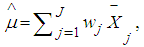 | (5) |
 is the weight for each group in the data distribution and
  is the mean of each group in the observed ordered data set. The t statistic for each of the group is obtained using the formula:
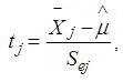 | (6) |
 is the mean for each of the independent groups,
  is the grand mean for all the independent groups with population j. The t statistic, with nj – 1 degrees of freedom. Denoting with
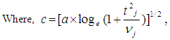
  the degree of freedom for each of the independent groups in the observed ordered data set. The t statistic obtained for the each of the groups and is converted to standard normal deviates by using the [7] normalization approximation in the [2] technique. The formula is expressed using:
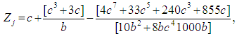 | (7) |
 | (8) |
 | (9) |
 | (10) |
3. The Winsorized Modified Alexander-Govern Test
- Consider an observed ordered data set:
 , with sample size n and group sizes j. Firstly, the median of the data set is obtained by selecting the middle value from the observations. The MAD estimator is the median of the set of the absolute values of the differences between each of the score and the median. It is the median of
  . Therefore, the median absolute deviation about the median
  estimator is obtained by using the formula below:
 | (11) |
 when sampling from a normal distribution. Outliers in a data distribution can be detected by using the formula below:
 | (12) |
 | (13) |
 represents the observed ordered random sample,
  is the median of the ordered random samples and
  is the median absolute deviation about the median. The value of K is 2.24. This value was introduced by [29] for detecting the presence of outliers in a data set, because it has a very small standard error, when sampling from a normal distribution. Equation (12) and (13) helps to define the MOM estimator used for detecting the presence of outliers in a data distribution. In this research, we modified the mean as a measure of the central tendency in Alexander-Govern test by replacing it with the Winsorized modified one step M-estimator (WMOM) as a central tendency measure for the test. The WMOM estimator is applied on the data distribution where the outlier detected value is replaced with the preceding value closest to the position the outlier is located. The WMOM estimator is obtained by averaging the Winsorized data distribution. It is expressed as:
 | (14) |
 | (15) |
 is the observed random sample and
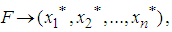
  is the Winsorized MOM estimator for the Winsorized data distribution. The standard error of WMOM is obtained by using the bootstrapping method. The bootstrapping algorithm for estimating the standard errors is expressed as below.Firstly, we chose B independent bootstrap samples defined as:
  Where each of these random samples comprises of n data values chosen with replacement from x expressed as:
 | (16) |
 | (17) |
 is not the real data set of x but it refers to a resampled version of x. In estimating the standard error of the bootstrap samples, the number of B falls within the range of (25 – 200). According to [6] bootstrap sample size of 50 is sufficient enough to give a reasonable estimate of the standard error of the MOM estimator. In this research, the same sample size was used to estimate the standard error of the MOM estimator.Secondly, we evaluate the bootstrap replication corresponding to each of the bootstrap sample define as:
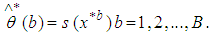 | (18) |
 by the sample standard deviation of the bootstrap (B) replications expressed as:
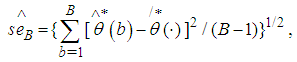 | (19) |
 The weight
  for the Winsorized data distribution for each of the independent groups is defined as:
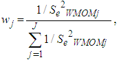 | (20) |
 is the squared-standard error of the Winsorized data distribution and is expressed as:
 | (21) |
 | (22) |
 is defined as the weight for the Winsorized data distribution, and
  is defined as the mean of the Winsorized data distribution.The t statistic for the Winsorized data distribution for each of the group is expressed using the formula:
 | (23) |
 ,
,  and
and  is the Winsorized MOM estimator, the total mean for the Winsorized data distribution and the standard error of the Winsorized data distribution data distribution respectively. In the [2] method, the
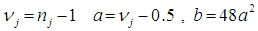
  value is converted to standard normal by using the [7] normalization approximation and the hypothesis testing of the Winsorized sample variance of the WMOM estimator for
  is defined as:
 For j = (j = 1, …,J)The normalization approximation formula for the Alexander-Govern method, using the Winsorized Modified One Step M-estimator is expressed as:
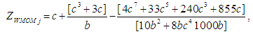 Where
Where 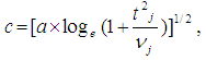
 The test statistic of the Winsorized Modified One Step M-estimator in Alexander-Govern test for all the groups in the observed ordered data sample is expressed as:
 | (24) |
4. To Evaluate the Efficiency and Reliability of the Tests Using Real Life Data
- A real life data which was obtained from [9] that comprises of three independent groups, namely: the group young, middle and old was used to evaluate the efficiency and reliability of the AG test and the AGWMOM test respectively.
|
|
|
|
|
 = 0.05, if the significant value of any of the three groups is greater than 0.05, then the data is considered to be normally distributed. Otherwise, if the significant value is less than 0.05, then the data distribution is non-normal.
|

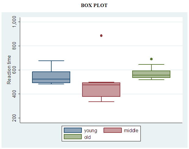 | Figure 1. Boxplots on reaction time against the young, middle and old groups |
|
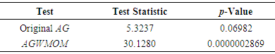
 = 0.05 level of significant. This shows that the AG test is not significant, since its p-value of 0.06982 > 0.05. While the test statistic value of the AGWMOM test produced a value of 30.1280, which is almost six times that of the AG test. The AGWMOM test has a p-value of 0.0000002869 at
  = 0.05 level of significant. The AGWMOM test is regarded as significant, since its p-value of 0.0000002869 is < 0.05 compared to the AG test. The standard error of the Winsorized AGMOM from the real life data for the young, middle and old group is far smaller compared to the standard error of the AG test from the original real life data.
5. Conclusions
- The AGWMOM test is more efficient and reliable in minimizing error as much as possible from the real life data, by making a replacement for the presence of outliers in the real life data with a smaller standard error in comparison to the AG test.
ACKNOWLEDGEMENTS
- I give God Almighty all the thanks, praises, worship, honor, power, adoration and glory for everything. He is the author of wisdom, knowledge and understanding. The Everlasting Father, the beginning and ending of everything. I also want to acknowledge and thank my blessed, wonderful, special, very caring and ever-dynamic parents in person of Mr. and Mrs. D.K.O. Tobi, for their constant encouragement, love, sacrifice, support and goodwill. I love and appreciate them very greatly.