-
Paper Information
- Paper Submission
-
Journal Information
- About This Journal
- Editorial Board
- Current Issue
- Archive
- Author Guidelines
- Contact Us
International Journal of Statistics and Applications
p-ISSN: 2168-5193 e-ISSN: 2168-5215
2016; 6(1): 23-34
doi:10.5923/j.statistics.20160601.04

Aradhana Distribution and Its Applications
 Abstract
 Reference
 Full-Text PDF
 Full-text HTML
Rama Shanker
Department of Statistics, Eritrea Institute of Technology, Asmara, Eritrea
Correspondence to: Rama Shanker , Department of Statistics, Eritrea Institute of Technology, Asmara, Eritrea.
| Email: |  |
Copyright © 2016 Scientific & Academic Publishing. All Rights Reserved.
This work is licensed under the Creative Commons Attribution International License (CC BY).
http://creativecommons.org/licenses/by/4.0/

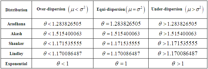
A new one parameter continuous distribution named “Aradhana distribution” for modeling lifetime data from biomedical science and engineering has been proposed. Its mathematical and statistical properties including its shape, moments, hazard rate function, mean residual life function, stochastic ordering, mean deviations, order statistics, Bonferroni and Lorenz curves, Renyi entropy measure, stress-strength reliability have been presented. The conditions under which Aradhana distribution is over-dispersed, equi-dispersed, under-dispersed are discussed along with the conditions under which Akash, Shanker, Lindley, and exponential distributions are over-dispersed, equi-dispersed and under-dispersed. The maximum likelihood estimation and the method of moments have been discussed for estimating its parameter. The applicability and the goodness of fit of the proposed distribution over Akash, Shanker, Lindley and exponential distributions have been discussed and illustrated with two real lifetime data - sets.
Keywords: Lindley distribution, Akash distribution, Shanker distribution, Mathematical and statistical properties, Estimation of parameter, Goodness of fit
Cite this paper: Rama Shanker , Aradhana Distribution and Its Applications, International Journal of Statistics and Applications, Vol. 6 No. 1, 2016, pp. 23-34. doi: 10.5923/j.statistics.20160601.04.
Article Outline
1. Introduction
- The statistical analysis and modeling of lifetime data are essential in almost all applied sciences including, biomedical science, engineering, finance, and insurance, amongst others. A number of one parameter continuous distributions for modeling lifetime data has been introduced in statistical literature including Akash, Shanker, exponential, Lindley, gamma, lognormal, and Weibull. The Akash, Shanker, exponential, Lindley and the Weibull distributions are more popular than the gamma and the lognormal distributions because the survival functions of the gamma and the lognormal distributions cannot be expressed in closed forms and both require numerical integration. Though each of Akash, Shanker, Lindley and exponential distributions have one parameter, the Akash, Shanker, and Lindley distribution has one advantage over the exponential distribution that the exponential distribution has constant hazard rate whereas the Akash, Shanker, and Lindley distributions has monotonically increasing hazard rate. Further, it has been shown by Shanker (2015a, 2015 b) that Akash and Shanker distributions gives much closer fit in modeling lifetime data than Lindley and exponential distributions. The probability density function (p.d.f.) and the cumulative distribution function (c.d.f.) of Lindley (1958) distribution are given by
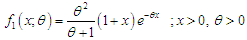 | (1.1) |
 | (1.2) |
 and a gamma distribution having shape parameter 2 and scale parameter
  with their mixing proportions
  and
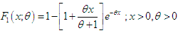
and  respectively. Detailed study about its various mathematical properties, estimation of parameter and application showing the superiority of Lindley distribution over exponential distribution for the waiting times before service of the bank customers has been done by Ghitany et al (2008). The Lindley distribution has been generalized, extended and modified along with their applications in modeling lifetime data from different fields of knowledge by different researchers including Zakerzadeh and Dolati (2009), Nadarajah et al (2011), Deniz and Ojeda (2011), Bakouch et al (2012), Shanker and Mishra (2013 a, 2013 b), Shanker and Amanuel (2013), Shanker et al (2013), Elbatal et al (2013), Ghitany et al (2013), Merovci (2013), Liyanage and Pararai (2014), Ashour and Eltehiwy (2014), Oluyede and Yang (2014), Singh et al (2014), Sharma et al (2015 a, 2015 b), Shanker et al (2015 a, 2015 b), Alkarni (2015), Pararai et al (2015), Abouammoh et al (2015) are some among others.Shanker (2015 a) has introduced one parameter Akash distribution for modeling lifetime data defined by its p.d.f.and c.d.f.
 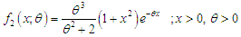 | (1.3) |
 | (1.4) |
 and a gamma distribution having shape parameter 3 and a scale parameter
  with their mixing proportions
  and
and  respectively. Shanker (2015 a) has discussed its various mathematical and statistical properties including its shape, moment generating function, moments, skewness, kurtosis, hazard rate function, mean residual life function, stochastic orderings, mean deviations, distribution of order statistics, Bonferroni and Lorenz curves, Renyi entropy measure, stress-strength reliability, amongst others. Shanker et al (2015 c) has detailed study about modeling of various lifetime data from different fields using Akash, Lindley and exponential distributions and concluded that Akash distribution has some advantage over Lindley and exponential distributions. Further, Shanker (2015 c) has obtained Poisson mixture of Akash distribution named Poisson-Akash distribution (PAD) and discussed its various mathematical and statistical properties, estimation of its parameter and applications for various count data-sets.The probability density function and the cumulative distribution function of Shanker distribution introduced by Shanker (2015 b) are given by
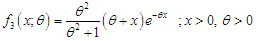 | (1.5) |
 | (1.6) |
 and a gamma distribution having shape parameter 2 and a scale parameter
  with their mixing proportions
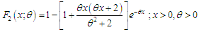
  respectively. Shanker (2015 b) has discussed its various mathematical and statistical properties including its shape, moment generating function, moments, skewness, kurtosis, hazard rate function, mean residual life function, stochastic orderings, mean deviations, distribution of order statistics, Bonferroni and Lorenz curves, Renyi entropy measure, stress-strength reliability , some amongst others. Further, Shanker (2015 d) has obtained Poisson mixture of Shanker distribution named Poisson-Shanker distribution (PSD) and discussed its various mathematical and statistical properties, estimation of its parameter and applications for various count data-sets.Although Akash, Shanker, Lindley and exponential distributions have been used to model various lifetime data from biomedical science and engineering, there are many situations where these distributions may not be suitable from theoretical or applied point of view.In search for a new lifetime distribution, we have proposed a new lifetime distribution which is better than Akash, Shanker, Lindley and exponential distributions for modeling lifetime data by considering a three-component mixture of an exponential distribution having scale parameter
  , a gamma distribution having shape parameter 2 and scale parameter
  , and a gamma distribution with shape parameter 3 and scale parameter
  with their mixing proportions
  respectively. The probability density function (p.d.f.) of a new one parameter lifetime distribution can be introduced as
 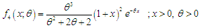 | (1.7) |
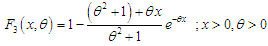
 | (1.8) |
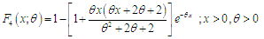
 are shown in figures 1 and 2.
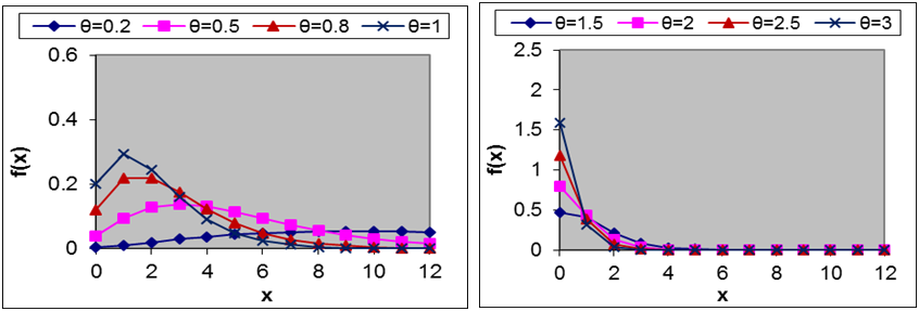 | Figure 1. Graph of the pdf of Aradhana distribution for different values of parameter  |
 | Figure 2. Graph of the cdf of Aradhana distribution for different values of parameter  |
2. Moment Generating Function, Moments and Related Measures
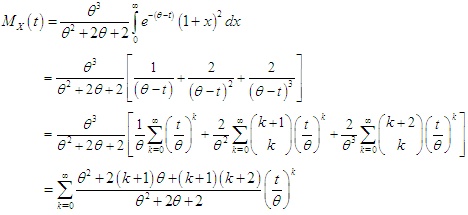
- The moment generating function of Aradhana distribution (1.7) can be obtained as
 Thus the
  moment about origin, as given by the coefficient of
  of Aradhana distributon (1.7) has been obtained as
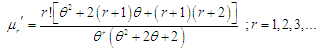 and so the first four moments about origin as
 Thus the moments about mean of the Aradhana distribution (1.7) are obtained as
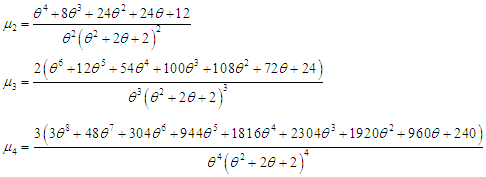 The coefficient of variation
  coefficient of skewness
  coefficient of kurtosis
  and Index of dispersion
  of Aradhana distribution (1.7) are thus obtained as
|

3. Hazard Rate Function and Mean Residual Life Function
- Let
 be a continuous random variable with p.d.f.
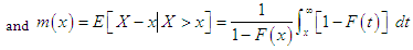
  The hazard rate function (also known as the failure rate function) and the mean residual life function of
  are respectively defined as
 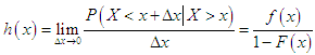 | (3.1) |
 | (3.2) |
 and the mean residual life function,
  of the Aradhana distribution (1.7) are obtained as
 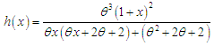 | (3.3) |
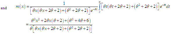 | (3.4) |
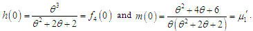 It is also obvious from the graphs of
 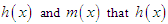 is an increasing function of
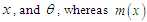 is a decreasing function of
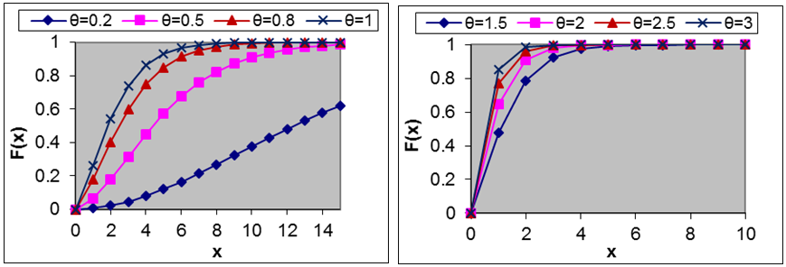
  The graphs of the hazard rate function and mean residual life function of Aradhana distribution (1.7) are shown in figures 3 and 4.
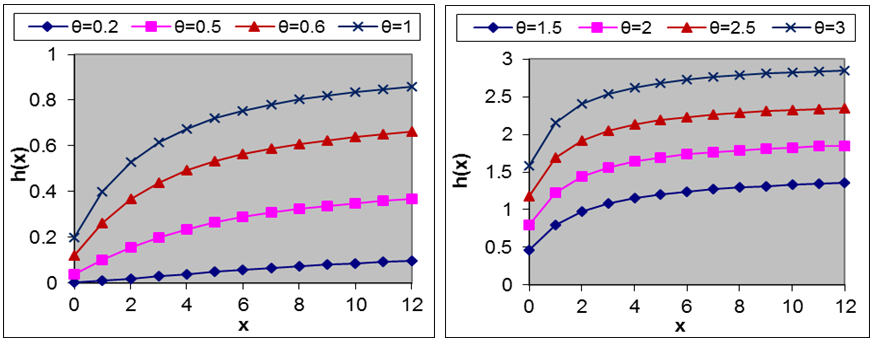 | Figure 3. Graph of hazard rate function of Aradhana distribution for different values of parameter  |
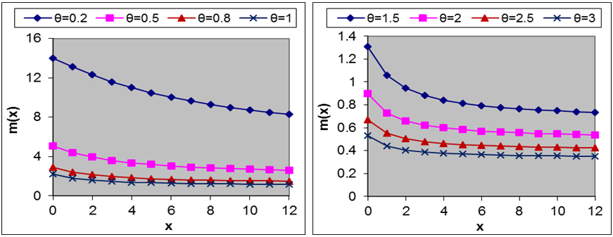 | Figure 4. Graph of mean residual life function of Aradhana distribution for different values of parameter  |
4. Stochastic Orderings
- Stochastic ordering of positive continuous random variables is an important tool for judging their comparative behavior. A random variable
 is said to be smaller than a random variable
  in the (i) stochastic order
  for all
  (ii) hazard rate order
  for all
  (iii) mean residual life order
  if
if  for all
  (iv) likelihood ratio order
  decreases in
  The following results due to Shaked and Shanthikumar (1994) are well known for establishing stochastic ordering of distributions
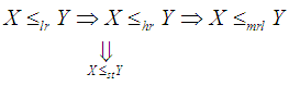 The Aradhana distribution is ordered with respect to the strongest ‘likelihood ratio’ ordering as shown in the following theorem:Theorem: Let
  Aradhana distributon
  and
and 
 Aradhana distribution
  . If
. If  then
then  and hence
  and
and  Proof: We have
  Now
Now  This gives
  Thus for
  This means that
  and hence
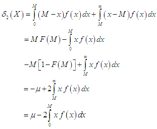
5. Mean Deviations
- The amount of scatter in a population is measured to some extent by the totality of deviations usually from their mean and median. These are known as the mean deviation about the mean and the mean deviation about the median and are defined as
 and
and  respectively, where
  and
and  The measures
  can be computed using the following simplified relationships
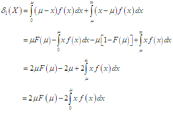 | (5.1) |
 | (5.2) |
 | (5.3) |
 | (5.4) |
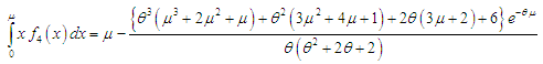
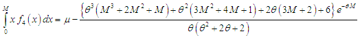
 and the mean deviation about median,
  of Aradhana distribution (1.7), after a little algebraic simplification, are obtained as
 | (5.5) |
 | (5.6) |
6. Order Statistics
- Let
 be a random sample of size
  from Aradhana distribution (1.7). Let
  denote the corresponding order statistics. The p.d.f. and the c.d.f. of the
  order statistic, say
  are given by
 and
and 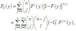 ,respectively, for
 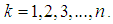 Thus, the p.d.f. and the c.d.f of
  order statistics of Aradhana distribution (1.7) are obtained as
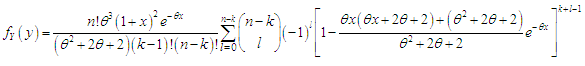 and
and 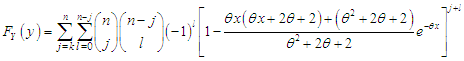
7. Bonferroni and Lorenz Curves
- The Bonferroni and Lorenz curves (Bonferroni, 1930) and Bonferroni and Gini indices have applications not only in economics to study income and poverty, but also in other fields like reliability, demography, insurance and medicine. The Bonferroni and Lorenz curves are defined as
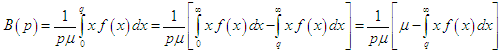 | (7.1) |
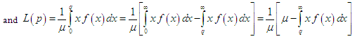 | (7.2) |
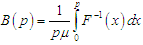 | (7.3) |
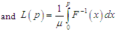 | (7.4) |
 The Bonferroni and Gini indices are thus defined as
 | (7.5) |
 | (7.6) |
 | (7.7) |
 | (7.8) |
 | (7.9) |
 | (7.10) |
 | (7.11) |
8. Renyi Entropy
- An entropy of a random variable
 is a measure of variation of uncertainty. A popular entropy measure is Renyi entropy (1961). If
  is a continuous random variable having probability density function
  then Renyi entropy is defined as
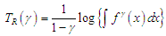 where
where  Thus, the Renyi entropy for the Aradhana distribution (1.7) can be obtained as
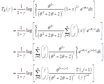
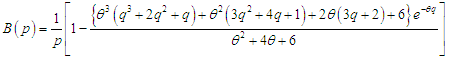
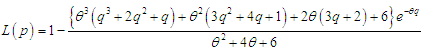
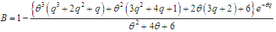
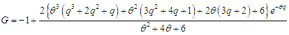
9. Stress-strength Reliability
- The stress - strength reliability describes the life of a component which has random strength
 that is subjected to a random stress
  . When the stress
  applied to it exceeds the strength
  , the component fails instantly and the component will function satisfactorily till
  . Therefore,
  is a measure of component reliability and is known as stress-strength reliability in statistical literature. It has wide applications in almost all areas of knowledge especially in engineering such as structures, deterioration of rocket motors, static fatigue of ceramic components, aging of concrete pressure vessels etc.Let
  be independent strength and stress random variables having Aradhana distribution (1.7) with parameter
  respectively. Then the stress-strength reliability
  can be obtained as
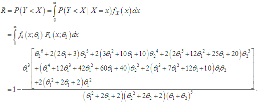 .
.10. Estimation of Parameter
10.1. Maximum Likelihood Estimation
- Let
 be a random sample from Aradhana distribution (1.7). The likelihood function, of Aradhana distribution (1.7) is given by
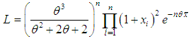 The natural log likelihood function is thus obtained as
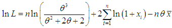 Now
Now 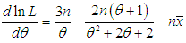 where
where  is the sample mean.The maximum likelihood estimate,
  is the solution of the equation
  and so it can be obtained by solving the following non-linear equation
 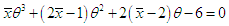 | (10.1.1) |
10.2. Method of Moment Estimation
- Equating the population mean of the Aradhana distribution to the corresponding sample mean, the method of moment (MOM) estimate,
 is same as given by equation (10.1.1).
11. Applications and Goodness of Fit
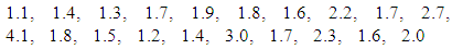
- The Aradhana distribution has been fitted to a number of lifetime data-sets relating to biomedical science and engineering. In this section, we present the fitting of Aradhana distribution to two real lifetime data- sets and compare its goodness of fit with the one parameter Akash, Shanker, Lindley and exponential distributions.Data set 1: The first data - set represents the lifetime’s data relating to relief times (in minutes) of 20 patients receiving an analgesic and reported by Gross and Clark (1975, P. 105). The data are as follows:
 Data set 2: The second data - set is the strength data of glass of the aircraft window reported by Fuller et al (1994)
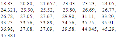 In order to compare the goodness of fit of Aradhana, Akash, Shanker, Lindley and exponential distributions,
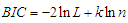
  AIC (Akaike Information Criterion), AICC (Akaike Information Criterion Corrected), BIC (Bayesian Information Criterion), K-S Statistics (Kolmogorov-Smirnov Statistics) for two real lifetime data - sets have been computed and presented in table 2. The formulae for computing AIC, AICC, BIC, and K-S Statistics are as follows:
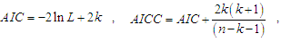
 and
and  where
where  the number of parameters,
  the sample size and
  is the empirical distribution function. The best distribution for modeling lifetime data is the distribution corresponding to lower values of
  AIC, AICC, BIC, and K-S statistics
|
 AIC, AICC, BIC, and K-S Statistics of the fitted distributions of data -sets 1 and 2
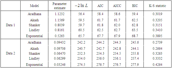
12. Conclusions
- A new one parameter lifetime distribution named, “Aradhana distribution” has been suggested for modeling lifetime data-sets from engineering and medical science. Its important mathematical and statistical properties including shape, moments, skewness, kurtosis, hazard rate function, mean residual life function, stochastic ordering, mean deviations, order statistics have been discussed. Further, expressions for Bonferroni and Lorenz curves, Renyi entropy measure and stress-strength reliability of the suggested distribution have been derived. The method of moments and the method of maximum likelihood estimation have also been discussed for estimating its parameter. Finally, the goodness of fit test using K-S Statistics (Kolmogorov-Smirnov Statistics) for two real lifetime data- sets have been presented to demonstrate the applicability and comparability of Aradhana, Akash, Shanker, Lindley and exponential distributions for modeling lifetime data - sets.
ACKNOWLEDGMENTS
- The author expresses his gratefulness to the anonymous reviewer for constructive comments.