Subhash Bagui1, Sikha Bagui2, Rohan Hemasinha1
1Department of Mathematics and Statistics, The University of West Florida, Pensacola, USA
2Department of Computer Science, The University of West Florida, Pensacola, USA
Correspondence to: Subhash Bagui, Department of Mathematics and Statistics, The University of West Florida, Pensacola, USA.
| Email: |  |
Copyright © 2016 Scientific & Academic Publishing. All Rights Reserved.
This work is licensed under the Creative Commons Attribution International License (CC BY).
http://creativecommons.org/licenses/by/4.0/

Abstract
In this article, we study the statistical classification of breast cancer of two well-known large breast cancer databases. We use various classification rules, such as linear, quadratic, logistic, k nearest neighbor (k-NN), and k rank nearest neighbor (k-RNN) rules and compare the performances. We also conduct feature analysis for both data sets using logistic regression model.
Keywords:
Classification rules, Discrimination, Linear and quadratic, Logistic, Nearest neighbor rules, Rank nearest neighbor rules, Classification error
Cite this paper: Subhash Bagui, Sikha Bagui, Rohan Hemasinha, The Statistical Classification of Breast Cancer Data, International Journal of Statistics and Applications, Vol. 6 No. 1, 2016, pp. 15-22. doi: 10.5923/j.statistics.20160601.03.
1. Introduction
According to the Centers for Disease Control (CDC) and Prevention, breast cancer is one of the most commonly diagnosed cancers and also one of the leading causes of death among American women [1]. Common kinds of breast cancer include ductal carcinoma, which begins in the cells that line the milk ducts in the breast, and lobular carcinoma, which begins in the lobes. In 2012 in US, according to CDC nearly 41,150 of the 224,147 women and 405 of the 2,125 men who developed breast cancer died [1].Currently, breast ultrasound, diagnostic mammogram, magnetic resonance imaging (MRI), and biopsy are the main tests used by doctors to diagnose breast cancer. Although some of the important signs of malignancy are captured by mammograms, detecting abnormalities based on visual analysis of the results is not always reliable. In fact, mammography has a 10% false positive rate and misses at least 20% of breast cancer cases [2]. Consequently, accurate detection of tumors calls for the aid of intelligent systems to eliminate visual inspection error.When mammographic abnormalities are found, they can only be definitively evaluated by a biopsy, which involves localizing the questionable area and removing tissues for further laboratory examination [3]. The crucial role of microscopic indicators in cancer diagnosis provides the motivation for the selection of cellular features to build the best predictive model. In this article, our aim is to find the best breast cancer model for each of the two large breast cancer data sets and to compare the performance of various classification rules on them. In section 2, we describe methodologies of various classification rules, such as linear, quadratic, logistic, k-NN, and k-RNN rules. In section 3, we implement the mentioned rules on two large data sets and describe the results obtained from these rules with error tables and graphical analysis. Finally, in Section 4 we make our conclusion.
2. Methodology
2.1. Linear and Quadratic Discrimination
Discrimination is a multivariate technique concerned with separating distinct sets of objects and allocating new objects to previously defined groups based on a set of features,  . Suppose there are
  groups,
  . If associated with each group
  there is a probability density function of the measurements of the form
  , where
  , then an appropriate rule for the allocation process would be to allocate the individual with vector of scores x to
  if
if  . In this study, we are concerned with only two cancer outcomes—malignant and benign. Let
  and
and  be two multivariate populations, and let
  and
and  be the density functions associated with the random vector
  for the two populations, respectively. The density functions are normally distributed with mean
  and covariance matrix,
  for
for  . If two populations have equal covariance,
  , then the joint density of
 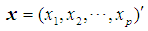 for populations
  is
is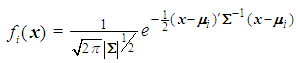 .Linear discrimination rule [3a]:By the linear classification rule, an object
  is classified into
  if
if  ,and, it is classified to
  otherwise. Quadratic discrimination rule [3a]:The quadratic classification rule is used when two groups have unequal covariance,
  ; an object
  is classified into
  if
if 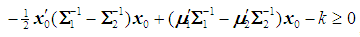 , where
 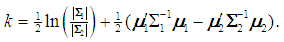 If
If  and
and  are unknown, then they may be replaced by their corresponding unbiased sample estimates,
  and
and  , respectively.The performance of a discriminant function can be evaluated by applying the rule to the data and then calculating the misclassification rate. A good method for estimating the misclassification rate of a discriminant function is by cross-validation, in which each record is used the same number of times for training and exactly once for testing.
2.2. Logistic Regression
Logistic regression is appropriate for a multivariable model whose outcome variable is binary, i.e. Y = 0 or 1. Instead of modeling the expected value of the response directly as a linear function of explanatory variables, logistic transformation is applied. Let Y = 1 be an event that occurs with probability  and let Y = 0 be an event that occurs with probability
  The odds of the event Y = 1 occurring is given by the ratio
  , and the logit is defined as the natural log of the odds. Thus, instead of modeling
  as a multiple linear regression function, (as
  is a binary variable), we model the logit (log of the odds) as a multiple linear regression function. This is more appropriate because this logit may assume values between
  depending on the range of
  . We now have
 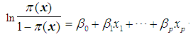 Next solving for
  , we obtain
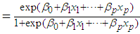 . The coefficients
  are estimated using maximum likelihood estimation.Logistic regression classification rule [3a]:An object
  is assigned to
  if the estimated odds is greater than 1, i.e. if
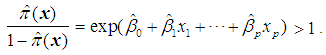 Equivalently, assign an object
  to
to  if the logit is greater than 0, i.e. if
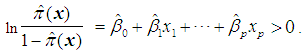
2.2.1. Model Selection Procedures
Testing the model involves obtaining the decomposition of the total variation in the response variable into that corresponding to variation accounted for by the model and the variations of the random deviations from the model. Suppose we fit a binary logistic model 
 to a set of data, where
  represents the probability of success. An F-statistic can be constructed to test the fit of the model. A significant F implies that we should reject the hypothesis that the regression coefficients β1, β2, … , βq all equal zero, or that none of the explanatory variables affects the response variable. This is usually not of primary concern; the investigator is more interested in assessing whether a subset of the explanatory variables can adequately explain the variation in the response variable. A more parsimonious model is easier to interpret, and it may reduce cost and the possibility of measurement error. The two commonly used methods for model selection are described below [3b].Forward selection The procedure of forward selection of variables begins with the fitting of a constant term, the mean, to the observations. Next, each of the possible variables is added to the model in succession, and the most significant one at a predetermined significant level is selected for inclusion. The remaining ones are then added in turn, and once again, only the most significant is selected. This process is repeated until no more variables meet entry criterion.Backward eliminationBackward elimination of variables begins with the full model, which contains all the possible explanatory variables. Each variable is deleted in turn, and the least significant one at a predetermined significant level is removed. This process is repeated until the simplest compatible model is obtained. Forward selection and backward elimination sometimes produce the same model, although this is not necessarily so.
2.3. k-NN (Nearest Neighbor) Classification Rule
The k-NN rule, proposed by Cover and Hart [4], is a modified version of Fix and Hodges’s NN rule [5, 6]. Let  and
and  be training samples from two given populations
  and
and  , and let
  be an observation known to originate from either
  or
or  to be classified between
  or
or  . Order the distances of all observations from
  using a distance function d. For a fixed integer k, the k-NN rule assigns the unknown observation
  to πi if the majority of the k nearest neighbors of
  come from
  , i = 1, 2. The distance functions used in this paper are described below.
2.3.1. Euclidean Distance
The Euclidean distance between points  and
and  is defined as
  where
where  is the dimension of the data.
2.3.2. Minkowski Distance ( -Norm Distance)
The Minkowski distance of order  between points
  and
and 
 is defined as
  . The 2-norm distance is the Euclidean distance.
2.3.3. Mahalanobis Distance
The Mahalanobis distance is a multivariate measure of the separation of a data set from a point in space. It takes into account the covariance among the variables in calculating distances, thereby correcting for the respective scales of the different variables. The Mahalanobis distance between two random vectors  and
and 
 from the same distribution with common covariance matrix
  is defined as
  . If the covariance matrix is the identity matrix, then the Mahalanobis distance reduces to the Euclidean distance.In this article, we apply the k-NN rule exclusively to the WBC data set. Due to the computational complexity of this rule, we only test a subset of the test set used in k-RNN classification. The test set was divided into five strata of equal size, and the k-NN rule was then used to classify a fixed number of points randomly selected from each group.
2.4. k-RNN (Rank Nearest Neighbor) Classification Rule
The k-RNN rule for multivariate data was first introduced by Bagui et al. [7]. Suppose we have two multivariate populations, an X-population,  and a Y- population,
  , and let us assume that
  follows a multivariate distribution with a mean of
  and covariance matrix
  of size
  and
and 
 follows a multivariate distribution with mean
  and covariance matrix
  of size
  . Let
. Let  be an observation known to be from either
  or
or  to be classified into
  or
or  . Suppose that only training data are available from both populations, and let
  and
and  be training samples from the two multivariate populations
  and
and  , respectively. A score function
 is used to obtain the pooled ranks of
  , and
, and  , where
  denotes the transpose of the mean vector
  and
and  denotes the inverse of the covariance matrix
  for i = 1, 2. This score function D(.) maps from
  to
to  , and it serves as a quadratic discriminant function between two populations. When
  , the score function serves as a linear discriminant function. In the case that
  and
and  are unknown, they may be replaced by their corresponding unbiased sample estimates,
  and
and  , respectively. k-RNN classification rule [7]After ranking the data in ascending order, consider k observations to the left of
  and k observations to the right of
  . If there are more
  than
than  among 2k RNN’s, then
  is classified into the X-population,
  . Similarly, if there are more
  than
than  , then
  is classified into the Y-population,
  . If there are exactly k
  and k
and k  , then
  can be classified into either of the two populations with probability ½ each. The k-RNN is also applied exclusively to the WBC data set in this article.
2.5. ROC Curve
The performance of a classification rule can be assessed by a receiver operating characteristic (ROC) curve, which is a graphical plot of the true positive rate (sensitivity) against the false positive rate (1-specificity). The point (0, 1) of the ROC space represents perfect classification—all true positives and no false positives. A good classification model should be as close as possible to this point, whereas a completely random guess would give a point along the main diagonal connecting the points (0, 0) and (1, 1). The maximum area under an ROC curve is 1, and this occurs only when the classification model is perfect.
3. Implementation and Results
We implement our methodologies on two large breast cancer databases, namely the Wisconsin breast cancer (WBC) database and the Wisconsin diagnostics breast cancer (WDBC) database.
3.1. Description of the Databases
Wisconsin Breast Cancer (WBC) database:The WBC database was created by Dr. William H. Wolberg, a physician at the University of Wisconsin Hospital, Madison [8] and donated by Olvi Mangasarian. The majority of the 699 cases, each identified by a sample code number, were recorded in January, 1989; the remaining cases, which include follow-up data in addition to new instances, were added to the database from October, 1989 to November, 1991. WBC [8] is a nine-dimensional data set with the following features: (i) Clump thickness; (ii) Uniformity of cell size; (iii) Uniformity of cell shape; (iv) Marginal adhesion; (v) Single epithelial cell size; (vi) Bare nuclei; (vii) Bland chromatin; (viii) Normal nucleoli; and (ix) Mitoses. These attributes have been used to represent instances.Patients were assigned an integer value from 1 to 10 for each of the aforementioned features, and each instance was classified as either benign or malignant. Approximately 65.5% of these instances were benign. A missing value for the bare nuclei attribute appeared in 16 instances, so we decided to exclude these incomplete observations. Also, 234 duplicate instances were deleted, leaving 449 data points (213 benign cases and 236 malignant cases) for our analyses. In 1990, Wolberg and Mangasarian [9] reported correct classification percentages of 93.5 and 92.2 using two different methods on the data set, composed of 369 instances at the time. Zhang [10] also studied this data set using 1-NN classification and by using only typical instances, with best accuracy results of 93.7% and 92.2%. Wisconsin Diagnostic Breast Cancer (WDBC) database:The WDBC database was obtained from W.H. Wolberg et al. of the University of Wisconsin, Madison [11, 12] and donated by Nick Street in 1995. Each of the thirty features, which describe characteristics of the cell nuclei present, was computed from a digitized image of a fine needle aspirate (FNA) of a breast mass [13, 14]. Approximately 62.7% (357 instances) of the 569 instances were diagnosed as benign, and the rest, malignant. The ten real-valued features that Wolberg et al. [13,14] considered for each cell nucleus are: (i) radius (mean of distances from center to points on the perimeter; (ii) texture (standard deviation of gray-scale values); (iii) perimeter; (iv) area; (v) smoothness (local variation in radius lengths); (vi) compactness (perimeter^2 / area - 1.0); (vii) concavity (severity of concave portions of the contour); (viii) concave points (number of concave portions of the contour); (ix) symmetry; and (x) fractal dimension (coastline approximation – 1.0).The authors [13, 14] then computed the mean, standard error, and worst mean (mean of the three largest values) of these features for each image, resulting in 30 features. Bennett and Mangasarian [15] created separating hyperplanes that use multisurface method-tree (MSM-T) and a classification method involving linear programming to find the three best features, which are Worst Area, Worst Smoothness, and Mean Texture. The estimated accuracy based on these three features was 97.5% using repeated 10-fold cross-validations.
3.2. Results
3.2.1. WBC database
Let the random variable  denote the benign population and the random variable
  denote the malignant population, both following a multivariate distribution. Let us denote the WBC data set by XWBC = XB
  XM, where XB is the set of benign cases and XM is the set of malignant cases. Disregarding the duplicate points and those with missing values, we have |XWBC| = 449, of which 213 are benign cases and 236 malignant cases. For k-RNN and k-NN purposes, we also partition XWBC into a training data set, XTr, and a test data set, XTe such that XWBC = XTr
  XTe and XTr
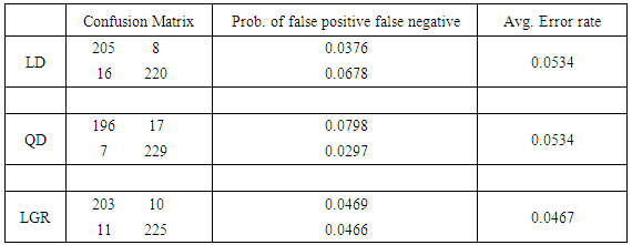
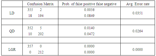
  XTe = Ø. The training set consists of 106 and 118 cases randomly selected from XB and XM, respectively, leaving 225 points (107 benign and 118 malignant) to be tested. Confusion matrices in the tables exhibit the number of correct classifications along the diagonal elements and the number of false positives and false negatives along the off-diagonal elements. We also report the probability of false negatives, probability of false positives, and the total (average) probability of misclassifications. The average error rates are calculated using prior probabilities of 0.4744 and 0.5256 for benign and malignant classes, respectively. Tables 1 and 2 show that linear and quadratic discrimination (LD & QD) yield the same average error rate. Also, logistic regression (LGR) returns a lower error rate than both types of discrimination However, quadratic discrimination results in the lowest false negative rate.
 Table 1. Summary of error rates for LD, QD, and LGR methods
 |
| |
|
Table 2. Summary of classification error with LGR model selection
 |
| |
|
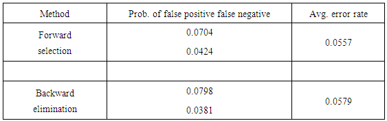
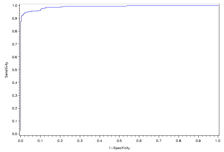
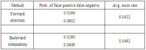
Next, we utilize the three model selection procedures described in section 2. Forward selection yields a model that includes the variables Clump Thickness, Uniformity of Cell Size, Marginal Adhesion, Bare Nuclei, Bland Chromatic, and Normal Nucleoli. Both backward elimination and stepwise selection result in a model that includes the aforementioned features but replaces Uniformity of Cell Size with Uniformity of Cell Shape. The average error rate for the second model is marginally higher, but we favor it for its lower false negative rate. We give more weight to the false negative rate in our considerations because overlooking a malignant case is much more detrimental than misdiagnosing a healthy patient. Figures 1 and 2 show the ROC curves for the full and reduced models, respectively. There is little discrepancy between the two curves, and both are close to the top left corner of the ROC space.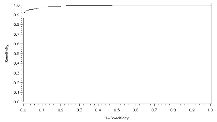 | Figure 1. ROC curve for full model under LGR |
 | Figure 2. ROC curve for reduced model under LGR |
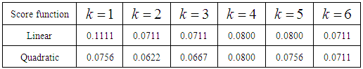
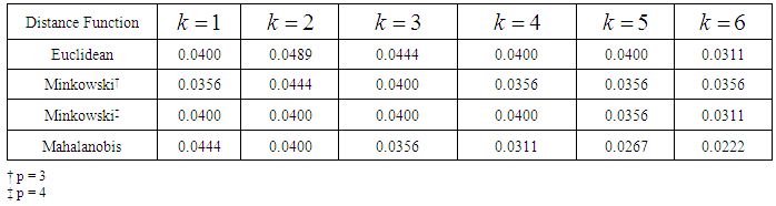
From the error rates summarized in Tables 3 and 4, we see that the k-NN classifier performs slightly better than the k-RNN classifier for the WBC data set. In k-RNN classification, the discrepancy between error rates calculated from linear and quadratic discrimination diminishes as the values of k increase from 1 to 6. In k-NN classification, the Mahalanobis distance function outperforms the p-norm distances for p = 2, 3, 4. Table 3. Error rates from XWBC classification using the k-RNN classifier
 |
| |
|
Table 4. Error rates from XWBC classification using the k-NN classifier
 |
| |
|
3.2.2. WDBC Database
In the following tables, we present confusion matrices, probability of false negatives, probability of false positives, and the total (average) probability of misclassifications as described in section 3.2.1. The average error rates are calculated using prior probabilities of 0.627 and 0.373 for benign and malignant classes, respectively. Table 5 shows that quadratic discrimination yields both a lower false negative rate and average error rate than linear discrimination. Once again, logistic regression performs better than both types of discrimination.Table 5. Summary of error rates from WDBCfor LD, QD, and LGR methods
 |
| |
|
The model under forward selection has lower average errors, computed with and without cross-validation, than that of the model obtained through backward elimination (Table 6). This model includes seven features—standard errors of Mean Radius and Compactness and worst mean values of Radius, Texture, Smoothness, Concavity, and Concave Points. Table 6. Summary of classification error from WDBC with LGR model selection
 |
| |
|
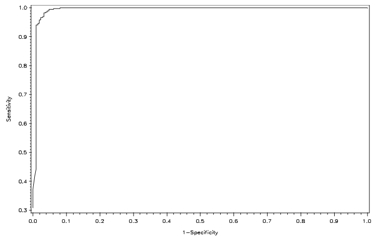
Figures 3 and 4 show the ROC curves for logistic regression of the full and reduced models, respectively. Both show higher correct classification rates.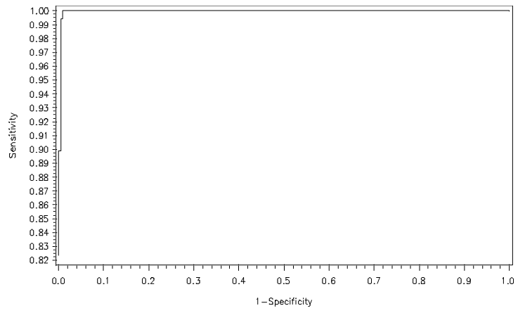 | Figure 3. ROC curve for full model under LGR |
 | Figure 4. ROC curve for reduced model under LGR |
4. Discussion and Conclusions
Through empirical study of the two data sets, we discovered that the WBC and WDBC models can be reduced from 9 and 30 variables to 6 and 7 variables, respectively. We also noted that logistic regression yields a lower classification error rate than linear and quadratic discrimination for both data sets. Furthermore, quadratic discrimination outperforms linear discrimination for both data sets. This is so because the covariances of the malignant and benign populations are unequal. Logistic regression resulted in no misclassifications for the full WDBC model and a 94.2% accuracy rate for the reduced model, which is only slightly lower than the best accuracy rate (97.5%) reported by Bennett and Mangasarian. The k-RNN classification rule did not perform as well as k-NN classification on XWBC, contrary to results from past research. The k-NN classification rule returned lower error rates than k-RNN for integer values less than 7 and also lower error rates than logistic regression for values greater than 3. The Mahalanobis distance function resulted in the lowest overall error rates as expected, since it is a statistical distance that takes into account the pooled covariance.
ACKNOWLEDGEMENTS
The first author’s research was supported by faculty catalyst awards at the University of West Florida (UWF). Part of the computations were done by Victoria Ding during her REU program at UWF. The authors would like to thank the referee for useful comments and suggestions on the earlier version of the paper.
References
| [1] | U.S. Cancer Statistics Working Group. United States Cancer Statistics: 1999-2010 Incidence and Mortality Web-based Report, Atlanta (GA): Department of Health and Human Services, Centers for Disease Control and Prevention, and National Cancer Institute; 2013. Available at: www.cdc.gov/uscs. |
| [2] | Wolberg, W.H., Biopsy for the “Abnormal” Mammogram; [updated 2000 June 27; cited 2007 Jul 26]; Retrieved July 26, 2007 from the world wide web: http://www.wisc.edu/wolberg/Laybrprob/biopsy.html. |
| [3] | A.D.A.M. Medical Encyclopedia [Internet]. Atlanta (GA): A.D.A.M., Inc.©2005. Biopsy; [updated 2006 Oct 16; cited 2007 Jul 26]; Retrieved July 26, 2007 from world wide web: http://www.nlm.nih.gov/medlineplus/ency/article/003416.htm. (3a) Johnson, R. and Wichern, D.W. (2007). Applied multivariate statistical analysis, Prentice Hall, New Jersey. (3b) Everitt, B. and Dunn, G. (2001). Applied multivariate data analysis, Wiley. |
| [4] | Cover, T.M. & Hart, P.E. (1967). Nearest neighbor pattern classification, IEEE Trans. Inf. Theory 13, 21-26. |
| [5] | Fix, E. & Hodges, J.L. (1951) Nonparametric discrimination: consistency properties: US Air Force School of Aviation Medicine, Report No. 4, Randolph Field, TX. |
| [6] | Silverman, B.W. & Jones, M.C. (1989). E. Fix and Hodges (1951): an important contribution to nonparametric discriminant analysis and density estimation. Int. Stat. Rev. 57, 233-247. |
| [7] | Bagui, S.C., Bagui, S.S., Pal, K., & Pal, N.R. (2003). Breast cancer detection using rank nearest neighbor classification rules, Pattern Recognition 36 (1), 25-34. |
| [8] | Mangasarian, O.L. & W. H. Wolberg, W.H. (1990). Cancer diagnosis via linear programming, SIAM News, 23(5), 1-18. |
| [9] | Wolberg, W.H. & Mangasarian, O.L. (1990). Multisurface method ofpattern separation for medical diagnosis applied to breast cytology, Proceedings of the National Academy of Sciences, U.S.A., 87, 9193-9196. |
| [10] | Zhang, J. (1992). Selecting typical instances in instance-based learning, Proceedings of the Ninth International Machine Learning Conference, Aberdeen, Morgan Kaufman, Scotland, 470-479. |
| [11] | Street, W.N., Wolberg, W.H., & Mangasarian, O.L. (1993). Nuclear feature extraction for breast tumor diagnosis. IS&T/SPIE 1993 International Symposium on Electronic Imaging: Science and Technology, San Jose, CA, Vol.1905, 861-870. |
| [12] | Mangasarian, O.L., Street, W.N., & Wolberg, W.H. (1995). Breast cancer diagnosis and prognosis via linear programming. Operations Research, 43(4), (1995), 570-577. |
| [13] | Wolberg, W.H., Street, W.N., & Mangasarian, O.L. (1994). Machine learning to diagnose breast cancer from fine-needle aspirates, Cancer Lett. 77, 163-171. |
| [14] | Wolberg, W.H., Street, W.N., D.M. Heisey, D.M. & Mangasarian, O.L. (1995). Computer- derived nuclear features distinguish malignant from benign breast cytology, Hum. Pathol. 26, 792-796. |
| [15] | Bennett, K.P. & O. L. Mangasarian, O.L. (1992). Robust linear programming discrimination of two linearly inseparable sets, Optimization Methods and Software 1, 23-34. |

 Abstract
 Reference
 Full-Text PDF
 Full-text HTML