-
Paper Information
- Paper Submission
-
Journal Information
- About This Journal
- Editorial Board
- Current Issue
- Archive
- Author Guidelines
- Contact Us
International Journal of Statistics and Applications
p-ISSN: 2168-5193 e-ISSN: 2168-5215
2015; 5(6): 338-348
doi:10.5923/j.statistics.20150506.08

Shanker Distribution and Its Applications
 Abstract
 Reference
 Full-Text PDF
 Full-text HTML
Rama Shanker
Department of Statistics, Eritrea Institute of Technology, Asmara, Eritrea
Correspondence to: Rama Shanker, Department of Statistics, Eritrea Institute of Technology, Asmara, Eritrea.
| Email: |  |
Copyright © 2015 Scientific & Academic Publishing. All Rights Reserved.
This work is licensed under the Creative Commons Attribution International License (CC BY).
http://creativecommons.org/licenses/by/4.0/

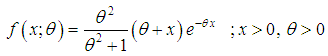
In this paper a new one parameter lifetime distribution named “Shanker distribution” for modeling lifetime data has been suggested. Various mathematical properties of the new distribution including its shape, moments, generating functions, hazard rate and mean residual life functions, stochastic ordering, order statistics, Renyi entropy measure, mean deviations, Bonferroni and Lorenz curves, and stress-strength reliability have been presented. The conditions of over-dispersion, equi-dispersion, and under-dispersion of Shanker distribution have been discussed. The method of maximum likelihood estimation and the method of moments have been discussed for estimating its parameter. The usefulness, applicability and superiority of the proposed distribution over exponential and Lindley distributions have been illustrated with three real lifetime data- sets.
Keywords: Moments, Hazard rate function, Mean residual life function, Mean deviations, Order statistics, Stress-strength reliability, Estimation of parameter, Goodness of fit
Cite this paper: Rama Shanker, Shanker Distribution and Its Applications, International Journal of Statistics and Applications, Vol. 5 No. 6, 2015, pp. 338-348. doi: 10.5923/j.statistics.20150506.08.
Article Outline
1. Introduction
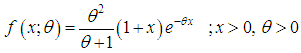
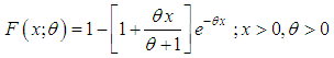
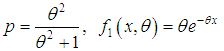
- A number of continuous distributions for modeling lifetime data such as exponential, Lindley, gamma, lognormal, and Weibull are available in statistical literature. The exponential, Lindley and the Weibull distributions are more popular than the gamma and the lognormal distributions for modeling lifetime data-sets because the survival functions of the gamma and the lognormal distributions cannot be expressed in closed forms and both require numerical integration. Though each of exponential and Lindley distributions has one parameter, the Lindley distribution has one advantage over the exponential distribution that the exponential distribution has constant hazard rate whereas the Lindley distribution has monotonically decreasing hazard rate.Lindley distribution, introduced in the context of Bayesian analysis as a counter example of fiducial statistics, having its probability density function (p.d.f.) and cumulative distribution function (c.d.f.)
 | (1.1) |
 | (1.2) |
 | (1.3) |
 and gamma
  distributions as follows:
 | (1.4) |
 and
and 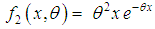 .The first derivative of (1.3) is obtained as
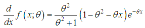 Thus
Thus  gives
gives  . From this it follows that (i) for
  ,
,  implies that
  is the unique critical point at which
  is maximized.(ii) for
  implies that
  is decreasing in
  .Therefore, the mode of the distribution (1.3) is given by
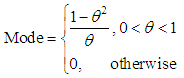 | (1.5) |
 | (1.6) |
 are shown in figures 1 and 2.
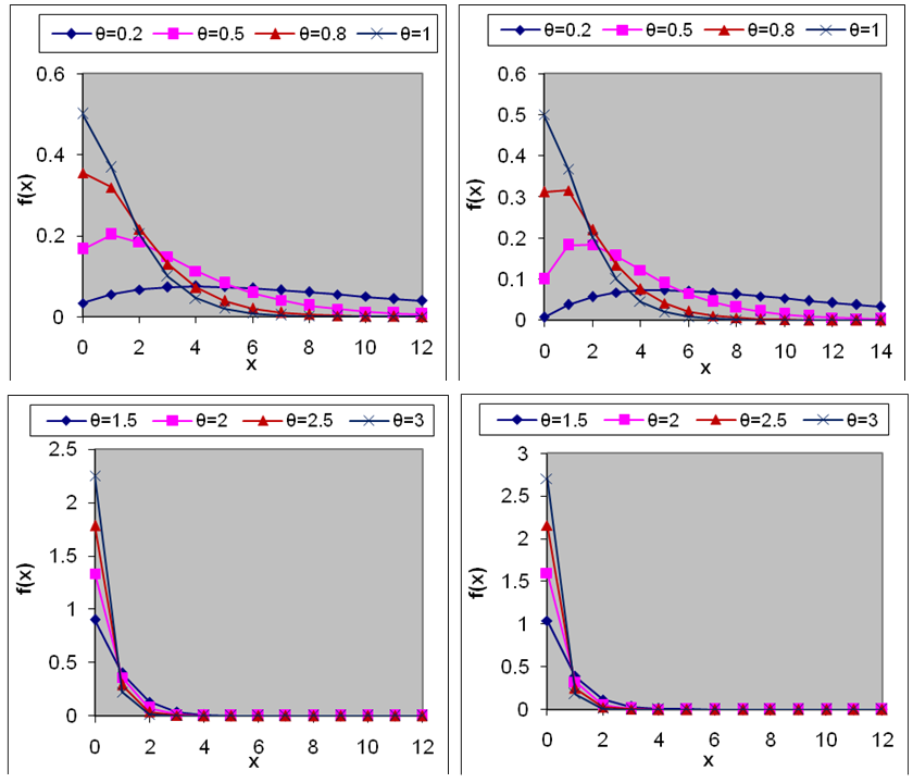 | Figure 1. Graphs of the pdf of Lindley and Shanker distributions for different values of parameter θ. Left hand side graphs are for Lindley distribution and right hand side graphs are for Shanker distribution |
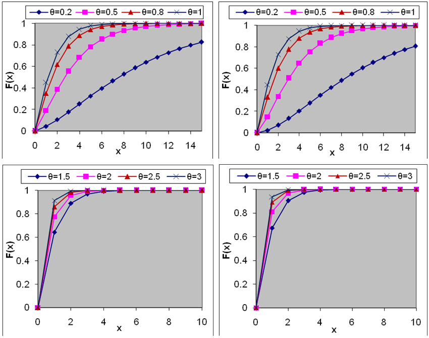 | Figure 2. Graphs of the cdf of Lindley and Shanker distribution for different values of parameter θ. Left hand side graphs are for Lindley distribution and right hand side graphs are for Shanker distribution |
2. Moments and Associated Measures
- The
 the moment about origin of Shanker distributon (1.3) has been obtained as
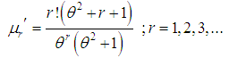 and so the first four moments about origin as
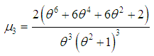
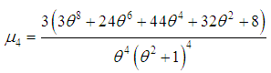
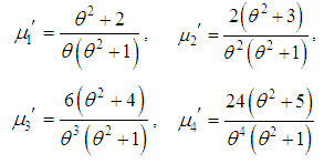 Thus the moments about mean of the Shanker distribution are as follows
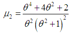
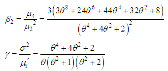
 The coefficient of variation
  , coefficient of skewness
  , coefficient of kurtosis
  and Index of dispersion
  of Shanker distribution are thus obtained as
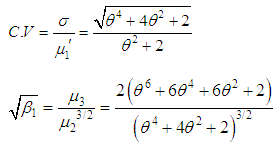
 It can be easily shown that Shanker distribution is over-dispersed
  , equi-dispersed
  and under-dispersed
  for
for 
 . It would be recalled that Lindley distribution is over-dispersed
 , equi-dispersed
  and under-dispersed
  for
for 
 while exponential distribution is over-dispersed
  , equi-dispersed
  and under-dispersed
  for
for  .
.3. Generating Functions
- The moment generating function
 , characteristic function
  , and cumulant generating function
  of Shanker distribution (1.3) are given by
 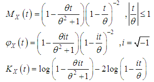 Using the expansion
 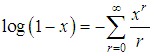 , we get
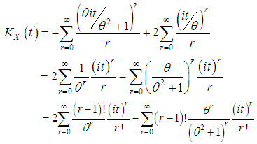 Thus the
  th cumulant of Shanker distribution is given by
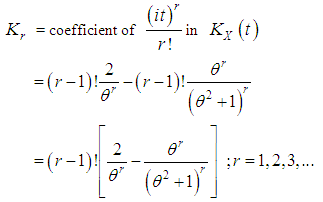 This gives
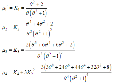 which are the same as obtained earlier.
4. Hazard Rate and Mean Residual Life Functions
- Let
 be a continuous random variable with p.d.f.
  and c.d.f.
  . The hazard rate function (also known as the failure rate function) and the mean residual life function of
  are respectively defined as
  | (4.1) |
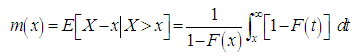 | (4.2) |
 and the mean residual life function,
  of Lindley distribution are given by
 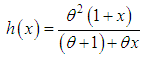 | (4.3) |
 | (4.4) |
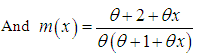
 and the mean residual life function,
  of the Shanker distribution are obtained as
 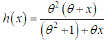 | (4.5) |
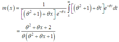 | (4.6) |
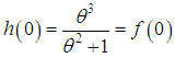 and
and 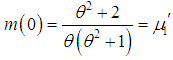 . It is also obvious from the graphs of
  and
and  that
that  is an increasing function of
  , and
, and  , whereas
  is a decreasing function of
  , and
, and  . The hazard rate function and the mean residual life function of the Shanker distribution show its flexibility over exponential and Lindley distributions. The graphs of the hazard rate function and mean residual life function of Lindley and Shanker distributions are shown in figures 3 and 4.
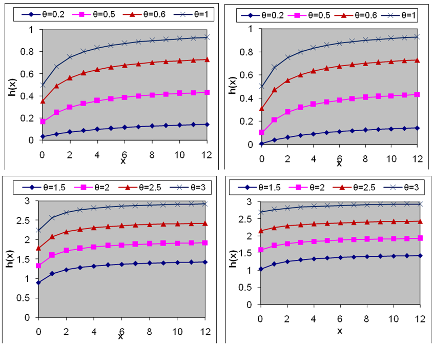 | Figure 3. Graph of hazard rate function of Lindley and Shanker distributions for different values of parameter θ. Left hand side graphs are for Lindley distribution and right hand side graphs are for Shanker distribution |
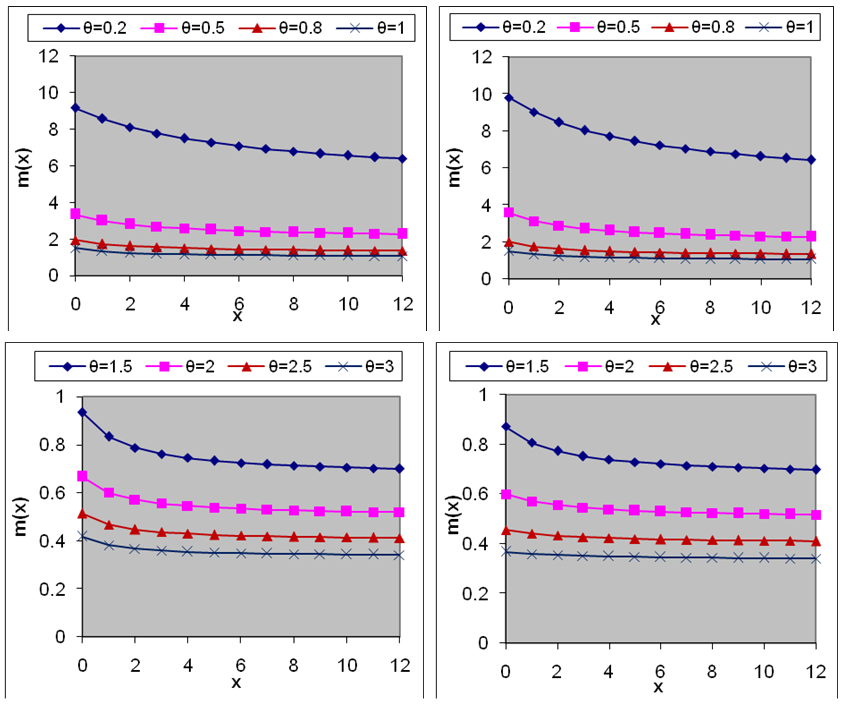 | Figure 4. Graphs of mean residual life function of Lindley and Shanker distributions for different values of parameter θ. Left hand side graphs are for Lindley distribution and right hand side graphs are for Shanker distribution |
5. Stochastic Orderings
- The stochastic ordering of positive continuous random variables is an important tool for judging their comparative behavior. A random variable
 is said to be smaller than a random variable
  in the (i) stochastic order
  if
if  for all
  (ii) hazard rate order
  if
if  for all
  (iii) mean residual life order
  if
if 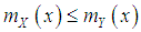 for all
  (iv) likelihood ratio order
  if
if  decreases in
  .The following stochastic ordering relationship given in Shaked and Shanthikumar (1994) are well known for stochastic ordering of distributions
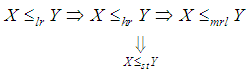 The Shanker distribution is ordered with respect to the strongest ‘likelihood ratio’ ordering which has been shown in the following theorem:Theorem: Let
  Shanker distributon
  and
and 
 Shanker distribution
  . If
. If  , then
  and hence
  ,
,  and
and  .Proof: We have
 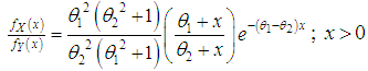 Now
Now  and
and 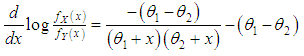 Thus for
  ,
,  . This means that
  and hence
  ,
,  and
and  .
.6. Distribution of Order Statistics
- Let
 be a random sample of size
  from Shanker distribution (1.3). Let
  denote the corresponding order statistics. The p.d.f. and the c.d.f. of the th order statistic, say
  are given by
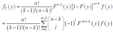 and
and 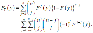 respectively, for
 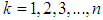 .Thus, the p.d.f. and the c.d.f of the th order statistics of Shanker distribution are obtained as
 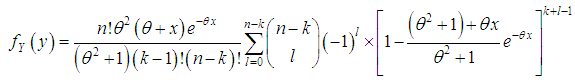 and
and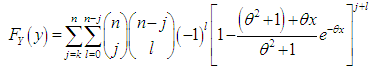
7. Renyi Entropy Measure
- The entropy of a random variable
 is the measure of variation of uncertainty. There are various entropy measures available in statistics literature but a popular entropy measure is Renyi entropy (1961). If
  is a continuous random variable having probability density function
  , then Renyi entropy is defined as
 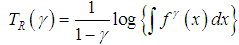 where
where 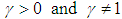 .Thus, the Renyi entropy for the Shanker distribution (1.3) can be obtained as
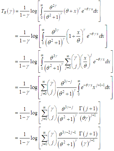
8. Mean Deviations from Mean and Median
- The amount of scatter in the population is measured to some extent by the totality of deviations usually from their mean and median and these are known as the mean deviation about the mean and the mean deviation about the median and are defined as
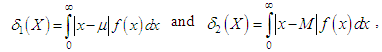 respectively, where
  and
and  . The measures
  and
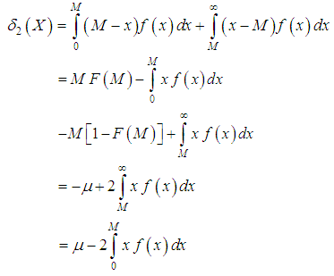
and  can be computed using the following simplified expressions
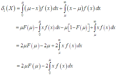 | (8.1) |
 | (8.2) |
 | (8.3) |
 | (8.4) |
 and
and  of Shanker distribution are obtained as
 | (8.5) |
 | (8.6) |
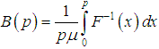
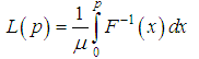
9. Bonferroni and Lorenz Curves and Indices
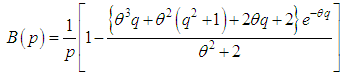
- The Bonferroni and Lorenz curves (Bonferroni, 1930) and Bonferroni and Gini indices have been used in economice to study income and poverty. Now a days, these curves and indices have many applications in other fields of knowledge including demography, reliability, insurance and medicine and engineering. The Bonferroni and Lorenz curves are defined as
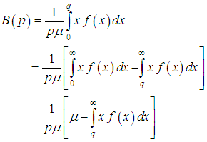 | (9.1) |
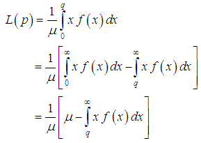 | (9.2) |
 | (9.3) |
 | (9.4) |
 and
and  .The Bonferroni and Gini indices are thus defined as
 | (9.5) |
 | (9.6) |
 | (9.7) |
 | (9.8) |
 | (9.9) |
 | (9.10) |
 | (9.11) |
10. Stress-Strength Reliability
- The stress- strength reliability describes the life of a component which has random strength
 that is subjected to a random stress
  . When the stress applied to it exceeds the strength
  , the component fails instantly and the component will function satisfactorily till
  . Therefore,
  is a measure of component reliability and it is known as stress-strength parameter in statistics literature. It has wide applications in almost all areas of knowledge especially in engineering such as structures, deterioration of rocket motors, static fatigue of ceramic components, aging of concrete pressure vessels etc.Let
  and
and  be independent strength and stress random variables having Shanker distribution (1.3) with parameter
  and
and  respectively. Then, the stress-strength reliability
  is obtained as
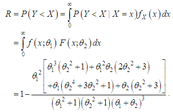
11. Estimation
11.1. Maximum Likelihood Estimate (MLE)
- Let
 be a random sample of size
  from Shanker distribution (1.3). The likelihood function,
  of (1.3) is given by
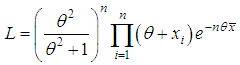 and so its log likelihood function is thus obtained as
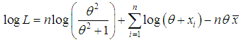 Now
Now 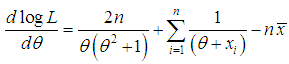 where
where  is the sample mean.The maximum likelihood estimate (MLE),
  of
of  is the solution of the equation
  and so it can be obtained by solving the following non-linear equation
 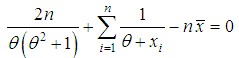 | (11.1.1) |
11.2. Method of Moment Estimate (MOME)
- Equating the population mean of the Shanker distribution to the corresponding sample mean, the method of moment estimate (MOME),
 of
of  is the solution of the following cubic equation
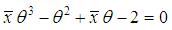 | (11.2.1) |
 is the sample mean.
 12. Applications
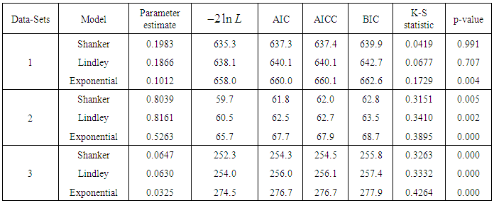
- The Shanker distribution has been fitted to a number of real lifetime data-sets and in almost all data-sets it gives better fit than exponential and Lindley distributions. In this section, we present the fittings of Shanker, Lindley and exponential distributions to three real lifetime data- sets to show the applicability and superiority of Shanker distribution over Lindley and exponential distributions.Data set 1: The first data - set represents the waiting times (in minutes) before service of 100 Bank customers and examined and analyzed by Ghitany et al (2008) for fitting the Lindley (1958) distribution. The data are as follows:0.8,0.8,1.3,1.5,1.8,1.9,1.9,2.1,2.6,2.7,2.9,3.1,3.2,3.3, 3.5,3.6,4.0,4.1,4.2,4.2,4.3,4.3,4.4,4.4,4.6,4.7,4.7,4.8,4.9,4.9,5.0,5.3,5.5,5.7,5.7,6.1,6.2,6.2,6.2,6.3,6.7,6.9,7.1,7.1,7.1,7.1,7.4,7.6,7.7,8.0,8.2,8.6,8.6,8.6,8.8,8.8,8.9,8.9,9.5,9.6,9.7,9.8,10.7, 10.9, 11.0, 11.0,11.1, 11.2, 11.2, 11.5, 11.9, 12.4, 12.5, 12.9, 13.0,13.1, 13.3, 13.6, 13.7, 13.9, 14.1, 15.4, 15.4, 17.3, 17.3, 18.1, 18.2, 18.4, 18.9, 19.0, 19.9, 20.6, 21.3,21.4, 21.9, 23.0, 27.0, 31.6, 33.1, 38.5.Data set 2: The second data - set represents the lifetime’s data relating to relief times (in minutes) of 20 patients receiving an analgesic and reported by Gross and Clark (1975, P. 105). The data are as follows:1.1, 1.4, 1.3, 1.7, 1.9, 1.8, 1.6, 2.2, 1.7, 2.7, 4.1, 1.8, 1.5, 1.2, 1.4, 3.0, 1.7, 2.3, 1.6, 2.0Data set 3: The third data set is the strength data of glass of the aircraft window reported by Fuller et al (1994)18.83, 20.80, 21.657, 23.03, 23.23, 24.05, 24.321, 25.50, 25.52, 25.80, 26.69, 26.77, 26.78, 27.05, 27.67, 29.90, 31.11, 33.20, 33.73, 33.76, 33.89, 34.76, 35.75, 35.91, 36.98, 37.08, 37.09, 39.58, 44.045, 45.29, 45.381 In order to compare exponential, Lindley and Shanker distributions,
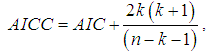
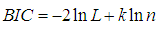
 , AIC (Akaike Information Criterion), AICC (Akaike Information Criterion Corrected), BIC (Bayesian Information Criterion), K-S Statistics (Kolmogorov-Smirnov Statistics) for three real lifetime data sets have been computed and presented in table 1. The formulae for computing AIC, AICC, BIC, and K-S Statistics are as follows:
  ,
,  ,
,  and
and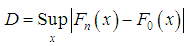 , where
  = the number of parameters,
  = the sample size and
  is the empirical distribution function. The best distribution which gives much closer fit to lifetime data-sets corresponds to lower
  , AIC, AICC, BIC, and K-S statistics
|
 ) introduced by Abouammoh et al (2015) and a two parameter Lindley distribution (with
  ) introduced by Shanker and Mishra (2013 a).
13. Concluding Remarks
- In the present paper a one parameter lifetime distribution named, “Shanker distribution” has been introduced. Its various mathematical properties including shape, moments and associated measures, hazard rate and mean residual life functions, stochastic ordering, mean deviations, and order statistics have been discussed. Further, expressions for Bonferroni and Lorenz curves, Renyi entropy measure and stress-strength reliability of the proposed distribution have been derived. The conditions of over-dispersion, equi-dispersion, and under-dispersion of Shanker distribution have been discussed along with the Lindley and exponential distributions. The method of moments and the method of maximum likelihood estimation have also been discussed for estimating its parameter. Finally, the goodness of fit test using K-S Statistics (Kolmogorov-Smirnov Statistics) for three real lifetime data- sets have been presented to demonstrate its applicability and superiority over exponential and Lindley distributions.
ACKNOWLEDGEMENTS
- The author is grateful to the anonymous reviewer for some helpful comments.