1. Introduction

Forecasting in time series analysis is extremity important both national economy and preproduction. Time series are commonly used in economic magnitude analysis, population forecasting and all other branches of science. So that it comes into prominence day after day. The criterion that increases the performance comes into prominence in various fields. Prediction modelings are used in many scientific fields. Interval-valued data represent uncertainty (for instance, confidence intervals), variability (minimum and maximum of daily temperature), etc. The field of interval analysis assumes that observations and estimations in the real world are usually incomplete and, consequently, do not precisely represent the real data. Interval-valued time series are interval-valued data collected in a chronological sequence. Maia and De Carvalho [1] stated that interval-valued time series could be seen in various different fields, e.g. economics (daily stock price of a company, which can be expressed as the lowest and highest trading prices over the day); engineering (the variation in an electric current, expressed by the lowest and highest intensities over a given day); medicine (diastolic and systolic blood pressure in a given day); weather (maximum and minimum rainfall in a month for a particular place); and relative humidity (also measured as the highest and lowest values in a given month).

Billard and Diday [2], Bock and Diday [3] and Diday and Noirhomme Fraiture [4] stated that interval-valued data have also been considered in the field of symbolic data analysis (SDA). This field is related to multivariate analysis, pattern recognition and artificial intelligence, and aims to extend classical exploratory data analysis and statistical methods to symbolic data. Symbolic data allow multiple (sometimes weighted) values for each variable and new variable types (set-valued, interval-valued and histogram valued variables) have been introduced. These new variables make it possible to take into account the variability and/or uncertainty present in the data. Symbolic Data Analysis (SDA) has been introduced by Billard and Diday [5] as a domain related to multivariate analysis, pattern recognition and artificial intelligence in order to introduce new methods and to extend classical data analysis techniques and statistical methods to symbolic data.

Various different approaches have been introduced for analyzing interval-valued data. A number of authors have considered neural network models in order to manage interval-valued data. For example, Beheshti et al. [6] propose a three-layer perceptron in which inputs, weights, biases and outputs are intervals, band show how to obtain the optimal weights and biases for a given training data set by means of interval computation algorithms. R. E. Patinŏ-Escarcina et al. [7] describe a one-layer perceptron for classification tasks in which inputs, weights and biases are represented by intervals. Roque et al. [8] propose and analyze a new multilayer perceptron model based on interval arithmetic which facilitates the handling of input and output interval data, but which has single valued rather than interval valued weights and biases.

In the field of SDA, several applications for managing interval-valued data have been provided: Ichino et al. [9] introduced a symbolic classifier as a region-oriented approach for symbolic interval data. Rasson and Lissoir [10] presented a symbolic kernel classifier based on dissimilarity functions suitable for symbolic interval data. Périnel and Lechevallier [11] proposed a tree-growing algorithm for classifying symbolic interval data. Bock [12] proposed several clustering algorithms for symbolic data described by interval variables and presented a sequential clustering and updating strategy for constructing a self-organizing map (SOM) to visualize symbolic interval data. Chavent and Lechevallier [13] proposed a dynamic clustering algorithm for interval data where the class representatives are defined by an optimality criterion based on a modified Hausdorff distance. Central tendency and dispersion measures are extended by Billard and Diday [5] and Chavent and Saracco [14]; factorial methods by Irpino [15]; multidimensional scaling by Groenen et al. [16]; hierarchical clustering by Gowda and Diday [17], Ichino and Yaguchi [18], Gowda and Ravi [19, 20], Chavent [21], and Guru et al. [22]; fuzzy by El-Sonbaty and Ismail [23], De Carvalho [24] and Yang et al. [25]; hard partition clustering by De Carvalho et al. [26], De Carvalho and Lechevallier [27,28], De Carvalho et al. [29], De Souza and De Carvalho [30], and Irpino and Verde [31]; regression by Lima Neto and De Carvalho [32]; and forecasting by Arroyo and Mat´e [33].

Souza and De Carvalho [34] presented partitioning clustering methods for interval data based on (adaptive and non-adaptive) city-block distances. More recently, De Carvalho et al. [35] have proposed an algorithm using an adequacy criterion based on adaptive Hausdorff distances. De Carvalho [36] proposed histograms for interval-valued data. Concerning factorial methods, Cazes et el. [37] and Lauro and Palumbo [38] proposed principal component analysis methods suitable for interval-valued data. According to Diday [39] statistical units described by interval data can be assumed as special cases of Symbolic Objects (SO). Currently, different approaches have been introduced to analyze symbolic interval data. Regarding univariate statistics, Bertrand and Goupil [40] and Billard and Diday [5] introduced central tendency and dispersion measures suitable for symbolic interval data. Billard and Diday [41] presented the first approach to fit a linear regression model on interval-valued data sets. Their approach consisted of fitting a linear regression model on the midpoint of the interval values assumed by the variables in the learning set and to apply this model on the lower and upper boundaries of the interval values of the explanatory variables to predict, respectively, the lower and upper boundaries of the interval values of the dependent variable. Lima Neto and De Carvalho [42] improved the former approach presenting a new method based on two linear regression models, the first regression model over the midpoints of the intervals and the second one over the ranges, which reconstruct the boundaries of the interval-values of the dependent variable in a more efficient way when compared with the Billard and Diday’s method. Palumbo and Verde [43] and Lauro et al. [44] generalized factorial discriminant analysis (FDA) to interval-valued data. Concerning interval-valued time series, Maia et al. [45] have introduced autoregressive integrated moving average (ARIMA), artificial neural network (ANN) as well as a hybrid methodology that combines both ARIMA and ANN models in order to forecast interval-valued time series. Silva [46] used copulas approach to the regression models for interval-valued data attack the problem from an optimization point of view. Maia and De Carvalho [1] introduced three approaches to forecasting interval-valued time series. The first two approaches are based on multilayer perceptron (MLP) neural networks and Holt’s exponential smoothing methods, respectively. In Holt’s method for interval valued time series, the smoothing parameters are estimated by using techniques for non-linear optimization problems with bound constraints. The third approach is based on a hybrid methodology that combines the MLP and Holt models. The practicality of the methods is demonstrated through simulation studies and applications using real interval-valued stock market time series.

This study examines the interval-valued time series which has been an ongoingness issue in time series. The study aims to obtain new time series forecasting methods using different combination of several analysis methods and modeling techniques and to determine the methods and models that provide the optimal accuracy by comparing the forecasting accuracy of the proposed methods. To do this, four real time series are used. These time series are Usage of Gold Exchange I-Istanbul (Weekday, Turkish Liras/US dollar), Usage of Gold Exchange II-Istanbul (Weekday, Turkish Liras/US dollar), Cost of Living Index (Wage Earners) (1995=100) and Selling Rate of Exchange-Euro (Exchange Selling). Obtained results represent the dependent variables in the variance analysis of our study. Independent variables involve forecasting methods. In the next section, brief information about interval-valued time series processing in time series analysis is given. By utilizing tables, Section 3 presents the results obtained from the implementation in which four real time series are analyzed. In the last section, the obtained results are summarized, interpreted and discussed.

2. Interval-Valued Time Series Processing

Maia and De Carvalho [1] reported that classical statistics and data analysis deal with individuals who are described by usual variables that assume a single value for a given individual: either a real value (for a quantitative variable) or a category from a set of alternatives (for either a nominal or an ordinal qualitative variable). Symbolic variables generalize this classical paradigm, as the value of a symbolic variable may be a subset of a set of categories, an interval of R, or a histogram for an underlying classical variable. In this paper, we are concerned with interval-valued variables. In the context of SDA, Bock and Diday [3] used an interval-valued variable X is a correspondence defined from Ω (the set of individuals) into R, such that, for each k ∈ Ω, X(k) = [a, b] ∈ ℑ, where ℑ = {[a, b] : a, b ∈ R, a ≤ b} is the set of closed intervals defined from R. Maia et al.[45] indicated that when interval-valued variables are collected in an ordered sequence over time, we say that we have an interval-valued time series. In the development of this work, we consider that, at each point in time (t = 1, 2, . . . , n), an interval is described as a two-dimensional vector with components in R representing the upper boundary and the lower boundary , with . Thus, an ITS (Interval-valued time series) is

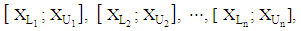where n denotes the number of intervals of the time series (sample size). Specifically, an observed interval at time t is it, and is represented as

Thus, an ITS is a set of intervals , each recorded at a specific time t and generally time equidistant.

We often come across interval-valued variables in practice. For instance, an interval may describe the smallest and largest values of a measurement for an individual over a day, or the range of monthly income values in a city. Fig. 1 illustrates two typical situation which an ITS arises. At the top of Fig. 1, the ITS on the right is the series of temperature intervals, which are obtained at each instant in time from the minimal and maximal values of the time series of temperatures on the left. At the bottom of Fig. 1, the ITS on the right is the series of intervals of stock prices, which are obtained at each instant in time from the highest and lowest trading values of the stock options recorded monthly.

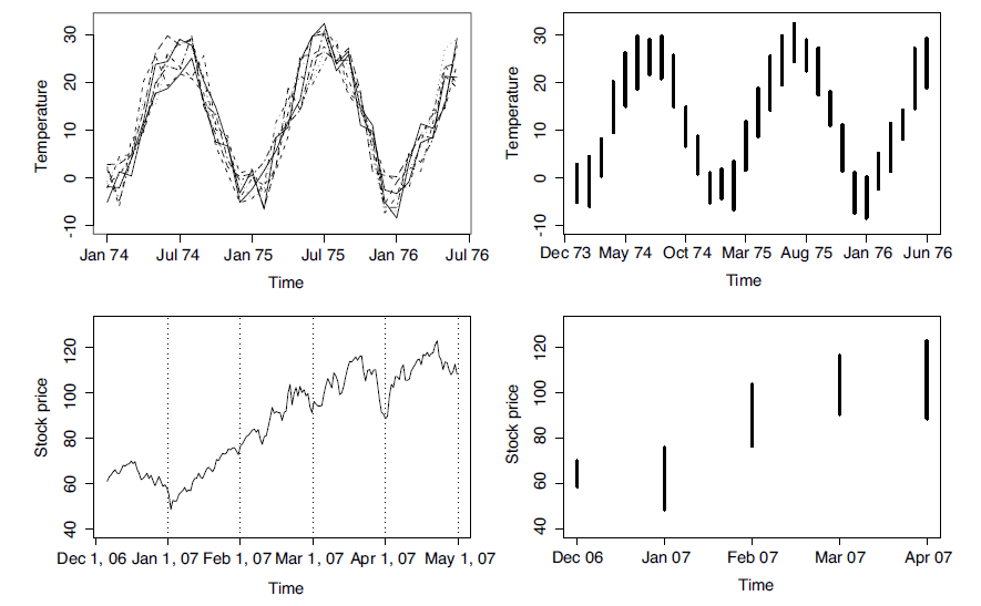Figure 1. Two interval-valued time series (right hand side) obtained from a set of usual time series (left hand side)

2.1. Constructing Models for Interval-Valued Time Series Forecasting

2.1.1. Approach 1

Maia et al. [45] suggest that the upper and lower bounds ( - the upper bounds of the interval, –the lower bounds of the interval) of interval-valued time series predicted by neural networks separately.

In approach 1, forecasts for the lower and upper bounds obtain from these models, respectively.

In the precedent expression, are a non-linear function determined by the neural networks, respectively.

2.1.2. Approach 2

Maia et al. [45] suggest that the upper and lower bounds of interval-valued time series predicted by neural networks together. In approach 2 forecasts for the lower and upper bounds obtain from this model. In this approach only one function determined by the neural networks and obtained the lower and upper bounds.

In the precedent expression is a non-linear function determined by the neural networks. In this approach, the inputs of neural networks the lower and the upper bounds of lagged variables of time series

outputs are values.

2.1.3. Approach 3

Lima Neto and De Carvalho [47] presented two time series. These are the interval centre series and the range interval series , respectively, represent the centre and the range interval series by,

and time series are analyzed by using feed forward neural networks, separately. In this circumstance, the forecasts of and time series obtained from two models given below.

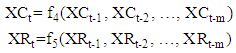In the methods presented here, and are respectively a non-linear function determined by the neural network of lagged variables of mid-point and range series. Thus, the values predicted by these models for the lower and upper bounds of the interval, given by.

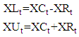
2.2. Modeling Techniques Used in Approaches

2.2.1. Box-Jenkins (ARIMA) Models

An often-used methodology in handling and predicting time series is known as the Box-Jenkins method or simply ARIMA. An autoregressive (AR) model is simply a model used to find an estimation of a variable based on previous input values of the variable. The actual equation for the AR model is as follows:

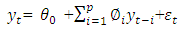where is the current value of the time series at time t. The (i=1,2,…,p) are the model parameters to be estimated. The model consists of three parts: a constant part , a random error part (white noise) and the AR summation. The parameter p represents the order of the model AR(p).

Autoregressive moving average (ARMA) models are created from a finite, linear combination of past values of the series and a finite linear combination of past errors. The particular model that will be used in the present paper, known as ARMA(p; q), is represented as follows:

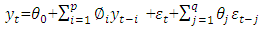where is the random error at time t; (i=1; 2; . . . ; p) and (j=1,2,…,q) are the model parameters to be estimated; p and q refer to the order of the model; the random errors are assumed to be independent and identically distributed with a zero mean and constant variance. In practice, one applies the ARMA process not to the original time series, but to the transformed time series. Often, the time series of differences is stationary despite the non-stationary of the underlying process. Stationary time series can be well estimated by the ARMA model. This leads to the definition of the ARIMA model:

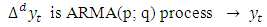
where is the d order differencing operator. The differencing operator is applied to the time series until it becomes stationary. Thus, an ARIMA (p; d; q) process models the stationary differences of the order d of the time series using the ARMA (p; q) process.

2.2.2. Neural Networks for Interval-Valued Time Series

Zhang et al. [48] mention that there is a huge range of different types of artificial neural networks, but the most popular type is the multilayer perceptron (MLP). In particular, feed-forward MLP networks with two layers (one hidden layer and one output layer) are often used for modeling and forecasting time series. Approaches based on artificial neural networks have also been proposed for the non-linear modeling of time series.

Kaastra and Boyd [49] proposed the relationship between the output, , and the inputs is as follows:

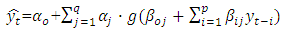in which and denote the weights of the connection between the constant input (bias) and the output, and between the bias and hidden nodes, respectively; and where and are the weights associated with each node; p is the number of inputs; q is the number of hidden nodes; and g denotes the transfer function used in the hidden layer. Transfer functions such as the logistic g(u) = 1/{1+exp(-u)} are commonly used for time series data, as they are non-linear and continuously differentiable, which are desirable properties for network learning.

In this paper, the neural network used is a MLP network for ITS processing , and is based on typical MLP networks for time series data. For ITS processing and forecasting, we use a MLP network with two feed-forward layers with 2p inputs (lagged intervals at t-1,…, t-p), q nodes in the hidden layer, and two output nodes, with each output corresponding to the forecasting of the boundaries, and .

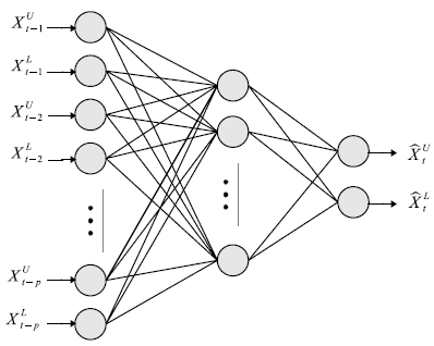Figure 2. Neural network for interval-valued time series processing, with 2p inputs and one hidden layer with q nodes and two outputs

Figure 2 displays the structure suitable for ITS processing. Note that the 2p inputs are used as a lagged ITS, i.e.,

There is a constant input unit, called a bias node, connected to every node in the hidden layer, as well as to the output nodes.

Let and be two-dimensional vectors,

for a network with one hidden layer of q nodes. The general prediction equation for computing forecasts of and (two outputs) using selected past intervals as the inputs is written in the following form:

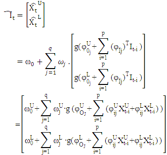where denotes the weights for the connections between the inputs (lagged intervals) and the hidden nodes; ω denotes the weights between the hidden nodes and the output nodes; and is the Hadamard product.

We train the MLP using conjugate gradient error minimization. The conjugate gradient approach finds the optimal weight vector along the current gradient by doing a line-search. Details of the conjugate gradient algorithm are given by Bishop [50].

2.2.3. Holt’s Method for Interval-Valued Time Series

The exponential smoothing method has become very popular due to its simplicity and good overall performance. Common applications range from business tasks (e.g., forecasting sales or stock fluctuations) to environmental studies (e.g., measurements of atmospheric components or rainfall data)—with typically no more a priori knowledge than the possible existence of trends in seasonal patterns. Such methods are sometimes also called naive, because no covariates are used in the models, i.e., the data are assumed to be self-explanatory. Their success is rooted in the fact that they belong to a class of local models that adapt their parameters to the data automatically during the estimation procedure, and therefore implicitly account for (slow) structural changes in the training data. Moreover, as the influence of new data is controlled by hyperparameters, this has the effect of smoothing the original time series.

Holt’s method proposed by Holt [51] is viewed as a common extension of the simple ES with an additional trend component. Two components must be updated each period—the level and the trend. The level is a smoothed estimate of the value of the data at the end of each period, while the trend is a smoothed estimate of the average growth at the end of each period. The specific formulae for Holt’s method are:

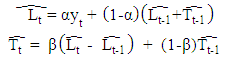where 0 < α, β < 1 are the smoothing parameters. In this model, α controls the length of the average for the estimation of the level and β controls the smoothing of the trend.

A straightforward approach to finding the optimal values of both α and β-constrained to be in the range (0, 1)—is to look for the parameter combination that minimizes the sum of squared errors of the one-stepahead predictions,

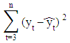where 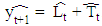. The starting values for and are typically taken as being and , respectively. More details are given by Gardner [52].

Numerous variations of the original exponential smoothing methods have been proposed. For example, Williams and Miller [53] proposed modifications for dealing with discontinuities. In this paper, the interval Holt’s exponential smoothing method (Holt’) follows a similar representation for usual quantitative data, and has the following form:

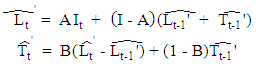where

and and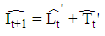

A and B denote the (2 × 2) smoothing parameter matrices,

and I is a (2 × 2) identity matrix.

The Holt’ method is given by

and

In the Holt’ method, the interpretation of the A and B parameter matrices is that they regulate the degree of smoothing. Thus, if A is an identity matrix (i.e. ), the curves are not smoothed at all, and if A is a null matrix (i.e. , the curves are absolutely smoothed; in fact, they show no variation at all. The parameter matrix B controls the smoothing of the trend. Moreover, the and parameters introduce information on the lower boundaries regarding the fitting of the upper boundaries, whereas the and parameters introduce information on the upper boundaries regarding the fitting of the lower boundaries.

In this method, the smoothing parameter matrices A and B, with elements constrained to the range (0, 1), can be estimated by minimizing the interval sum of squared one-step-ahead forecast errors:

The start vectors for and are typically taken to be and , respectively. Based on the above objective function, we may write the estimation of the smoothing parameter matrices as a constrained nonlinear programming problem, formulated as:

This is the method presented for estimating the optimal weight matrix for the Holt model intervals and for the prediction of ITS. The solution of this problem can be obtained using the limited memory BFGS method for bound constrained optimization (L-BFGS-B), developed by Byrd et al. [54] This method allows box constraints, that is, each parameter can be given lower and upper boundaries. It is based on the gradient projection method, and a quasi-Newton approach is used: the Broyden-Fletcher-Goldfarb-Shanno (BFGS) algorithm. The main goal of the BFGS algorithm is to use an approximate Hessian rather than the true Hessian. Nocedal and Wright [55] provided a comprehensive reference for the previous algorithms. The L-BFGS-B algorithm is implemented in the R software package by R Development Core Team [56].

2.2.4. Vector Autoregressive Models (VAR)

According to Füss [57] in ARIMA models we only derive the actual value from past values for an endogenous variable. However, there is often no theoretical background available. Therefore, we can use Vector Autoregressive (VAR) Models. The single equation approach explains an endogenous variable (e.g. private consumption) by a range of other variables (e.g., disposal income, property, interest rate) Assumption: Explanatory variables are exogenous. But macroeconomic variables are often not exogenous (endogenity problem). In theory exists no assumptions about the dynamic adjustment. Dynamic modeling of the consumption function, e.g. adjustment of consumption behavior to substantial income, occurs only slowly. Multivariate (linear) time series models eliminate both problems. Development of a variable is explained by the development of potential explanatory variables. Value is explained by its own history and simultaneously by considering various variables and their history. E.g. dependency of the long-term interest rate from the short run interest rate: is difficult in univariate time series analysis, because one would need estimations of the development of short run interest rate. Therefore, it is not possible to make good forecast out of such a model. In contrast to a bivariate model, where both, the history of long and short term interest rate are taken into consideration.

With vector autoregressive models it is possible to approximate the actual process by arbitrarily choosing lagged variables. Thereby, one can form economic variables into a time series model without an explicit theoretical idea of the dynamic relations.

2.2.4.1. Modeling of a VAR(1)-Models

Füss [57] stated that the most easy multivariate time series model is the bivariate vector autoregressive model with two dependent variables and where t = 1, ..., T. The development of the series should be explained by the common past of these variables. That means, the explanatory variables in the simplest model are and . The VAR(1) with lagged values for every variable is determined by:

Matrix Notation:

Assumptions about the Error Terms:

1. The expected residuals are zero:

2. The error terms are not autocorrelated:

Interpretation of VAR Models:

VAR-Models themselves do not allow us to make statements about causal relationships. This holds especially when VAR-Models are only approximately adjusted to an unknown time series process, while a causal interpretation requires an underlying economic model. However, VAR-Models allow interpretations about the dynamic relationship between the indicated variables.

2.2.4.2. VAR(p)-Models with more than two Variables

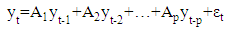
An VAR(p)-Model, with p variables, is given as:

If one wants to expand the equation with a trend, intercept or seasonal adjustment, it will be necessary to augment the vector which includes all the deterministic components, and the matrix B (VARX-Model):

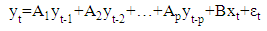Estimation of VAR-Models Specifications:

• Determination of endogenous variables according to economic theory, empirical evidence and experience.

• Transformation of time series (take logs or log-returns).

• Insert seasonal component, especially for macro data.

• Control for deterministic terms.

Determination of Lag Length:

The determination of lag length is a trade-off between the curse of dimensionality and abbreviate models, which are not appropriate to indicate the dynamic adjustment. If the lag length is to short, autocorrelation of the error terms could lead to apparently significant and inefficient estimators. Therefore, one would receive wrong results. With the so called curse of dimensionality we understand, that even with a relatively small lag length a large number of parameters if required. On the other hand, with increasing number of parameters, the degrees of freedom decrease, which could possibly result in significant of inefficient estimators.

Information Criteria:

The idea of information criteria is similar to the trade-off discussed above. On the one hand, the model should be able to reflect the observed process as precise as possible (error terms should be as small as possible) and on the other hand, to many variables lead to inefficient estimators. Therefore, the information criteria are combined out of the squared sum of residuals and a penalty term for the number of lags. In detail, for T observations we chose the lag length p in a way that the reduction of the squared residuals after augmenting lag p+1, is smaller than the according boost in the penalty term.

Squared residuals:

Penalty terms:

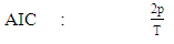
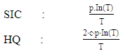with constant c > 1.

3. Implementation

The time series which are used in implementation obtained from internet site of Central Bank of the Turkish Republic. These data sets are described below.

Set1: Usage of Gold Exchange I-Istanbul (Weekday, TL/US dollar) between 03/01/2000 and 31/12/2011 dates.

Set2: Usage of Gold Exchange II-Istanbul (Weekday, TL/US dollar) between 03/01/2000 and 31/12/2011 dates.

Set3: Cost of Living Index (Wage Earners) (1995=100) between 03/01/2000 and 31/12/2011 dates.

Set4: Selling Rate of Exchange-Euro (Exchange Selling) between 03/01/2000 and 31/12/2011 dates.

The data of this time series are used in the implementation. This series have the lowest (US/ounce), the highest (US/ounce), centre (US/ounce) and range (US/ounce) values. To compare the methods, Root Mean Square Error (RMSE), Mean Absolute Percentage Error (MAPE), Theil’s interval statistics (U’) and interval average relative variance (ARV’) values are calculated by using the following formulas.

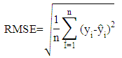
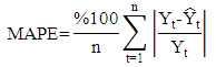
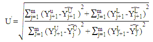
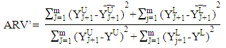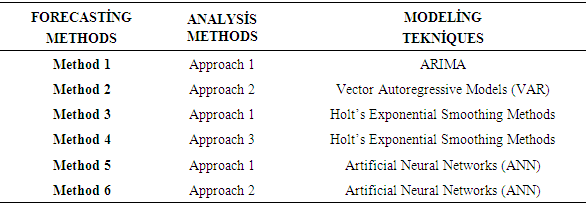
where is the actual value; is the predicted value; n is the number of data; m is the number of fitted intervals; is the t-th fitted interval; is the sample average interval; is upper boundary averages and lower boundary averages.

Forecasting methods compose of different combinations of several analysis methods and modeling techniques. Experimental study has done by using these different combinations. The data of experimental study are obtained by analyzing the interval-valued time series via forecasting methods. These values represent the dependent variables in the variance analysis of our study. The dependent variables measures accuracy of forecast outcomes and these are performance criterions. These performance criterions are Root Mean Square Error (RMSE), Mean Absolute Percentage Error (MAPE), Theil's Interval Statistics (U') and Interval Average Relative Variance (ARV') values. Independent variables involved eight forecasting methods. Kruskal-Wallis H test, multivariate statistical hypothesis test, was applied to evaluate the performance. Pairwise comparisons of the methods were performed using Mann-Whitney U-test. The study aimed to determine the methods and models that provide the optimal accuracy by comparing the forecasting accuracy of the proposed methods.

Additionally, the answer of the question that “which methods providing better forecasting results?” and their pros and cons were examined. In analysis stage, MATLAP, SPSS, EVIEWS and EXCEL are used. Programs are written in MATLAB programming language. The use of the methods and the contents of the methods are summarized in Table 1.

Table 1. The use of the methods and the contents of the methods

These methods are applied to four real interval-valued time series. The data of our experimental study were obtained by analyzing the interval-valued time series via forecasting methods. The obtained results are examined by using Kruskal-Wallis H and Mann-Whitney U nonparametric hypothesis tests. The reason of using nonparametric hypothesis test is that samples do not have Normal Distribution. And, median is preferred as a location parameter.

4. Emprical Results

4.1. Method 1

In this forecasting method, we are used Approach 1 as analysis method and ARIMA as modeling technique. We analyzed four interval-valued time series via forecasting methods. The obtained results are below.

Table 2. The obtained results for Usage of Gold Exchange I-Istanbul (Weekday, Turkish Liras/US Dollar)

Table 3. The obtained results for Usage of Gold Exchange II-Istanbul (Weekday, Turkish Liras/US Dollar)

Table 4. The obtained results for Cost of Living Index (Wage Earners) (1995=100)

Table 5. The obtained results for Selling Rate of Exchange-Euro (Exchange Selling)

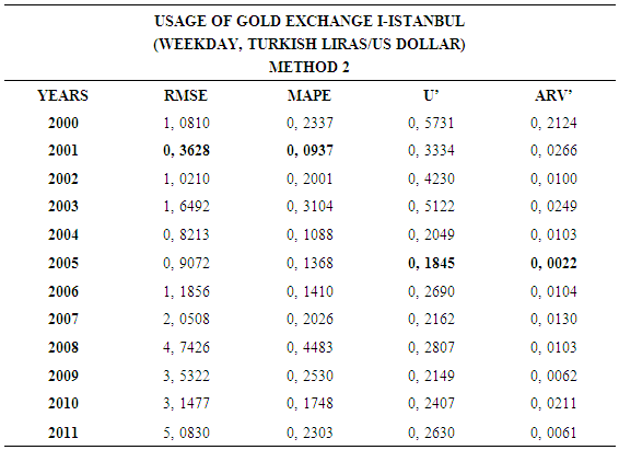
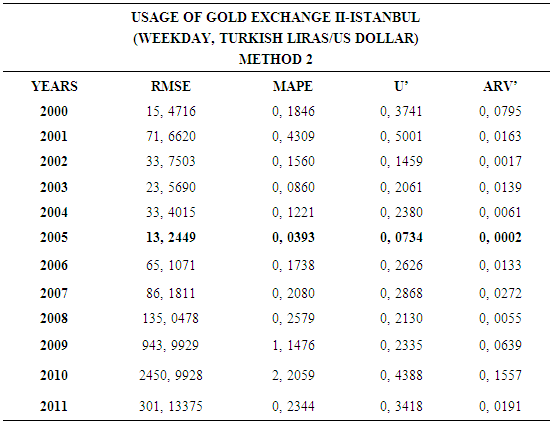
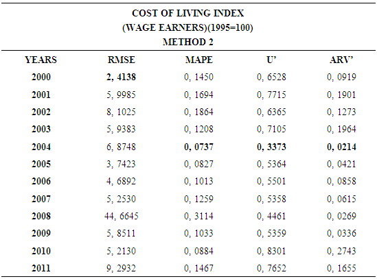
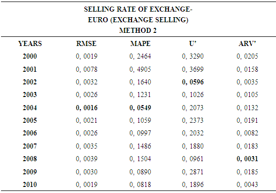
4.2. Method 2

In this forecasting method, we are used Approach 2 as analysis method and Vector Autoregressive Models (VAR) as modeling technique. We analyzed four interval-valued time series via forecasting methods. The obtained results are below.

Table 6. The obtained results for Usage of Gold Exchange I-Istanbul (Weekday, Turkish Liras/US Dollar)

Table 7. The obtained results for Usage of Gold Exchange II - Istanbul (Weekday, Turkish Liras/US Dollar)

Table 8. The obtained results for Cost of Living Index (Wage Earners) (1995=100)

Table 9. The obtained results for Selling Rate of Exchange-Euro (Exchange Selling)

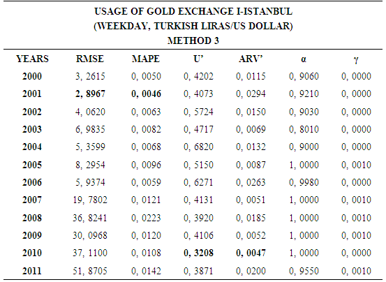
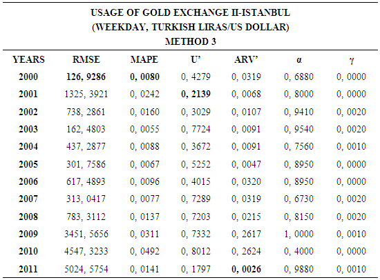
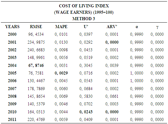
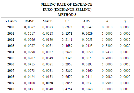
4.3. Method 3

In this forecasting method, we are used Approach 1 as analysis method and Holt’s Exponential Smoothing Methods as modeling technique. We analyzed four interval-valued time series via forecasting methods. The obtained results are below.

Table 10. The obtained results for Usage of Gold Exchange I-Istanbul (Weekday, Turkish Liras/US Dollar)

Table 11. The obtained results for Usage of Gold Exchange II-Istanbul (Weekday, Turkish Liras/US Dollar)

Table 12. The obtained results for Cost of Living Index (Wage Earners) (1995=100)

Table 13. The obtained results for Selling Rate of Exchange-Euro (Exchange Selling)

4.4. Method 4

In this forecasting method, we are used Approach 3 as analysis method and Holt’s Exponential Smoothing Methods as modeling technique. We analyzed four interval-valued time series via forecasting methods. The obtained results are below.

Table 14. The obtained results for Usage of Gold Exchange I-Istanbul (Weekday, Turkish Liras/US Dollar)

Table 15. The obtained results for Usage of Gold Exchange II-Istanbul (Weekday, Turkish Liras/US Dollar)

Table 16. The obtained results for Cost of Living Index (Wage Earners) (1995=100)

Table 17. The obtained results for Selling Rate of Exchange-Euro (Exchange Selling)

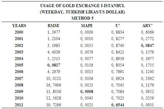
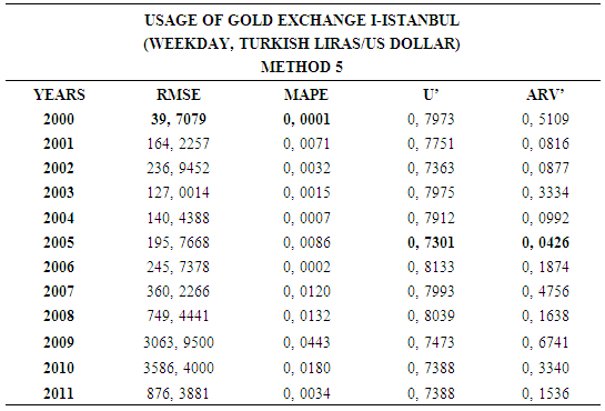
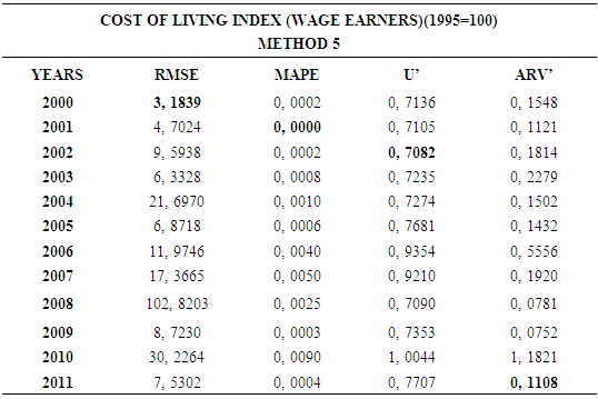
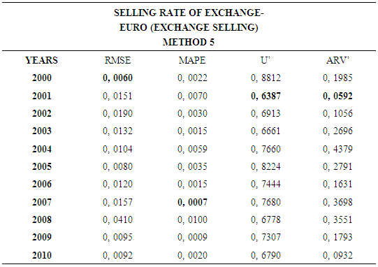
4.5. Method 5

In this forecasting method, we are used Approach 1 as analysis method and Artificial Neural Networks (ANN) as modeling technique. We analyzed four interval-valued time series via forecasting methods. The obtained results are below.

Table 18. The obtained results for Usage of Gold Exchange I-Istanbul (Weekday, Turkish Liras/US Dollar)

Table 19. The obtained results for Usage of Gold Exchange II-Istanbul (Weekday, Turkish Liras/US Dollar)

Table 20. The obtained results for Cost of Living Index (Wage Earners) (1995=100)

Table 21. The obtained results for Selling Rate of Exchange-Euro (Exchange Selling)

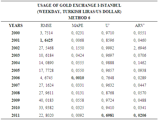
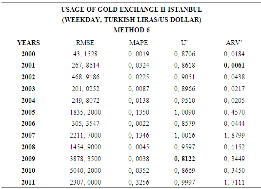
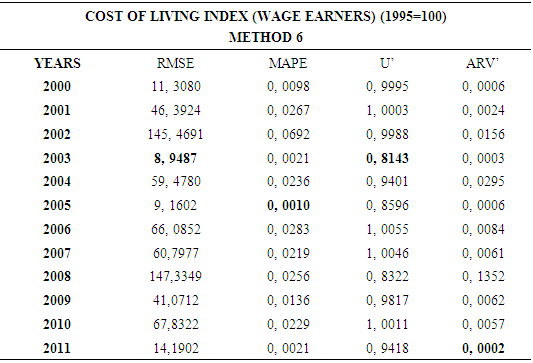
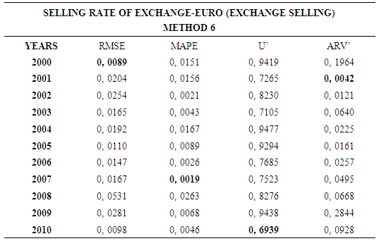
4.6. Method 6

In this forecasting method, we are used Approach 2 as analysis method and Artificial Neural Networks (ANN) as modeling technique. We analyzed four interval-valued time series via forecasting methods. The obtained results are below.

Table 22. The obtained results for Usage of Gold Exchange I-Istanbul (Weekday, Turkish Liras/US Dollar)

Table 23. The obtained results for Usage of Gold Exchange II-Istanbul (Weekday, Turkish Liras/US Dollar)

Table 24. The obtained results for Cost of Living Index (Wage Earners) (1995=100)

Table 25. The obtained results for Selling Rate of Exchange-Euro (Exchange Selling)

These values represent variables in the variance analysis of our study. The obtained results are analyzed by using statistical analysis. Kruskal-Wallis H test and Mann-Whitney U-test are applied to evaluate the performance.

Table 26. The best methods of performance criterias

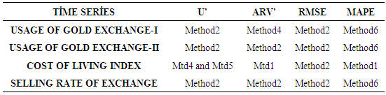
5. Conclusions and Discussion

This study examined the interval-valued time series which is an ongoingness issue in time series. Daily time series data are used as a data set. Different forecasting methods are proposed. The data of experimental study are obtained by analyzing the interval-valued time series via forecasting methods. These values represent the dependent variables in the variance analysis of our study. The obtained results are examined by using Kruskal-Wallis H and Mann-Whitney U nonparametric hypothesis tests. As a result of study, it can be said that, VAR model is more suitable for forecasting. The evaluation of the forecasting performance of the methods revealed that Method 2 which uses Approach 2 as analysis method and Vector Autoregressive Models (VAR) as modeling technique provide the highest forecast accuracy and closest results to the actual values. The superiority of VAR models is that variables do not pose a problem.