-
Paper Information
- Previous Paper
- Paper Submission
-
Journal Information
- About This Journal
- Editorial Board
- Current Issue
- Archive
- Author Guidelines
- Contact Us
International Journal of Statistics and Applications
p-ISSN: 2168-5193 e-ISSN: 2168-5215
2015; 5(6): 302-316
doi:10.5923/j.statistics.20150506.06

Reliability Analysis Using the Generalized Quadratic Hazard Rate Truncated Poisson Maximum Distribution
 Abstract
 Reference
 Full-Text PDF
 Full-text HTML
M. A. El-Damcese1, Dina A. Ramadan2
1Mathematics Department, Faculty of Science, Tanta University, Tanta, Egypt
2Mathematics Department, Faculty of Science, Mansoura University, Mansoura, Egypt
Correspondence to: Dina A. Ramadan, Mathematics Department, Faculty of Science, Mansoura University, Mansoura, Egypt.
| Email: |  |
Copyright © 2015 Scientific & Academic Publishing. All Rights Reserved.
This work is licensed under the Creative Commons Attribution International License (CC BY).
http://creativecommons.org/licenses/by/4.0/

In this paper, a new five-parameter lifetime distribution with failure rate is introduced for maximum reliability time in generalized linear hazard rate truncated poisson distribution. We obtain several properties of the new distribution such as its probability density function, its reliability and failure rate functions, quantiles and moments. Furthermore, estimation by maximum likelihood and inference are discussed. In the end, Application to real data set is given to show superior performance versus at least five of the known lifetime models.
Keywords: Failure rate, Generalized linear hazard rate truncate Poisson maximum distribution, Reliability, Order statistics, Residual life function, Maximum likelihood
Cite this paper: M. A. El-Damcese, Dina A. Ramadan, Reliability Analysis Using the Generalized Quadratic Hazard Rate Truncated Poisson Maximum Distribution, International Journal of Statistics and Applications, Vol. 5 No. 6, 2015, pp. 302-316. doi: 10.5923/j.statistics.20150506.06.
Article Outline
1. Introduction
- In reliability, many phenomena are modeled by statistical distributions. The probability distribution of the time -to-failure of a device can be characterized by the failure rate or hazard function.There are some parametric models that have successfully served as population models for failure times arising from a wide range of products and failure mechanisms. The distributions with Decreasing Failure Rate (DFR) property are studied in the works of Lomax (1954), Proschan (1963), Barlow et al. (1963), Barlow and Marshall (1964)-(1965), Marshall and Proschan (1965), Cozzolino (1968), Dahiya and Gurland (1972), McNolty et al. (1980), Saunders and Myhre (1983), Nassar (1988), Gleser (1989), Gurland and Sethuraman (1994), Adamidis and Loukas (1998), Kus (2007), and Tahmasbi and Rezaei (2008).For modeling the reliability and survival data with Increasing Failure Rate (IFR) property or bathtub failure rate, numerous hazard functions are proposed by different researches that most of them are based on Weibull distribution. Muldholkar and Srivastava (1993) proposed an Exponentiated Weibull family for analyzing bathtub failure-rate data. A model based on adding two Weibull distributions is presented by Xie and Lai (1995). Bebbington et al. (2007) proposed a new two-parameter distribution which is a generalization of the Weibull. Recently, Gupta et al. (2008) introduced another member of the Weibull family, which is called as the 'flexible Weibull distribution'. Recently, many new distributions, generalizing well-known distributions used to study lifetime data, have been introduced. Mudholkar and Srivastava (1993) presented a generalization of the Weibull distribution called the exponentiated (generalized)-Weibull distribution, GWD. The generalized exponential distribution, GED, introduced by Gupta and Kundu (1999). Nadarajah and Kotz (2006) introduced four exponentiated type distributions: the exponentiated gamma, exponentiated Weibull, exponentiated Gumbel. Sarhan and Kundu (2009) presented a generalization of the linear hazard rate distribution called the generalized linear hazard rate distribution, GLFRD. Sarhan et al. (2008) obtained Bayes and maximum likelihood estimates of the three parameters of the generalized linear hazard ratedistribution based on grouped and censored data. Recently, Sarhan (2009) introduced a generalization of the quadratic hazard rate distribution called the generalized quadratic hazard rate distribution (GQHRD).This paper is organized as follows: a new IFR distribution is obtained for maximum survival time by mixing generalized quadratic hazard rate and geometric distribution. Various properties of the proposed distribution are discussed in Section 3, 4 and 5. Rényi and Shannon entropies of the GQHRTPM distribution are given in Section 6. Residual and reverse residual life functions of the GQHRTPM distribution are discussed in Section 7. Section 8 is devoted to the Bonferroni and Lorenz curves of the GQHRTPM distribution. The maximum likelihood estimation procedure is presented. Fitting the GQHRTPM model to real data set indicate the flexibility and capacity of the proposed distribution in data modeling. In view of the density and failure rate function shapes, it seems that the proposed model can be considered as a suitable candidate model in reliability analysis, biological systems, data modeling, and related fields.
2. The Maximum Survival Time Distribution
- Let
 be a random sample from the generalized quadratic hazard rate distribution with Cumulative Density Function (cdf)
 and Z is a random variable from truncate at zero Poisson distribution with probability mass function as follows:
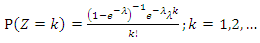 | (1) |
 By assuming that the random variables
  and Z are independent and defining
  then, the marginal distribution of X, for
  is
is 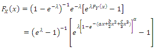 | (2) |
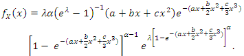 | (3) |

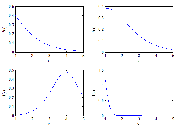 | Figure 1. Probability density function for GQHRTPMD from different values for a, b and c |
3. Reliability Analysis
- The reliability function (R) of the Generalized Quadratic Hazard Rate Truncated Poisson Maximum distribution is denoted by
 also known as the survivor function and is defined as
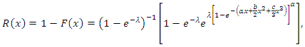 | (4) |
 | (5) |
 the hazard function is either increasing (if b > 0) or constant (if b = 0 and a >0);● when
  the hazard function should be:(1) increasing if b >0; (2) upside-down bath-tub shaped if b <0; and● if
  then the hazard function will be: (1) decreasing if b = 0 or (2) bath-tub shaped if b ≠ 0.
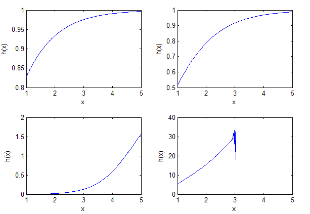 | Figure 2. The hazard rate function (HRF) for GQHRTPM from different values for a,b and c |
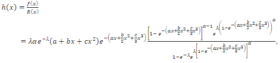
 is the probability of failure per unit of time, distance or cycles. These failure rates are defined with different choices of parameters in Figure 2. The cumulative hazard function of the Generalized Quadratic Hazard Rate Truncated Poisson Maximum distribution is denoted by
  and is defined as
 | (6) |
4. Statistical Analysis
4.1. The Median and Mode
- It is observed as expected that the mean of
 cannot be obtained in explicit forms. It can be obtained as infinite series expansion so, in general different moments of
  Also, we cannot get the quantile
  of
of  in a closed form by using the equation
 . Thus, by using Equation (2), we find that
 | (7) |
 can be obtained from (7), when
  as follows
 | (8) |
 can be obtained as a solution of the following nonlinear equation.
 | (9) |
4.2. Moments
- The following theorem 1 gives the
 moment of
  Theorem 1. If has
  the moment
  is given as follows for

 | (10) |
 Substituting (3) into the above relation, we get
 | (11) |
 is
is We get
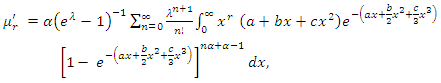 | (12) |
 for x, then by using the binomial series expansion of
  given by
 We get
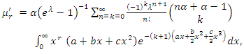 | (13) |
 and
and  are
are | (14) |
 | (15) |
 | (16) |
 | (17) |
4.3. The Moment Generating Function
- The moment generating function
 of the GQHRTPM distribution
  has the following form
 | (18) |
 | (19) |
5. Order Statistics
- The order statistics have many applications in reliability and life testing. The order statistics arise in the study of reliability of a system.Let
 be a simple random sample from
  with cumulative distribution function and probability density function as in (2) and (3), respectively. Let
  denote the order statistics obtained from this sample. In reliability literature,
  denote the lifetime of an
  system which consists of
  independent and identically components. Then the pdf of
  is given by
 | (20) |
 | (21) |
 | (22) |
 | (23) |
 | (24) |
 | (25) |
 , the last order statistics as
  and median order
5.1. Distribution of Minimum, Maximum and Median
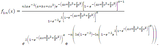
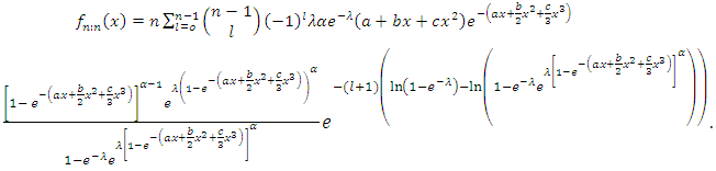
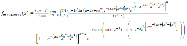
- Let
 be independently identically distributed order random variables from the GQHRTPM distribution having first, last and median order probability density function are given by the following
 | (26) |
 | (27) |
 | (28) |
 | (29) |
 | (30) |
 | (31) |
6. Rényi and Shannon Entropies
- If X is a random variable having an absolutely continuous cumulative distribution function
 and probability distribution function
  then the basic uncertainty measure for distribution F (called the entropy of F) is defined as
 Statistical entropy is a probabilistic measure of uncertainty or ignorance about the outcome of a random experiment, and is a measure of a reduction in that uncertainty. Numerous entropy and information indices, among them the Rényi entropy, have been developed and used in various disciplines and contexts. Information theoretic principles and methods have become integral parts of probability and statistics and have been applied in various branches of statistics and related fields. Entropy has been used in various situations in science and engineering. The entropy of a random variable Y is a measure of variation of the uncertainty. For a random variable with the pdf f, the Rényi entropy is defined by
 | (32) |
 is
is | (33) |
 | (34) |
 for x, then by using the binomial series expansion of
  and
and  given by
 | (35) |
 | (36) |
 and
and  are
are | (37) |
 | (38) |
 | (39) |
 | (40) |
 This is a special case derived from
7. Residual Life Function of the GQHRTPM Distribution
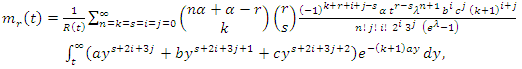
- Given that a component survives up to time t ≥ 0, the residual life is the period beyond t until the time of failure and defined by the conditional random variable X −t|X > t. The mean residual life (MRL) function is an important function in survival analysis, actuarial science, economics and other social sciences and reliability for characterizing lifetime. Although the shape of the failure rate function plays an important role in repair and replacement strategies, the MRL function is more relevant as the latter summarizes the entire residual life function, whereas the former considers only the risk of instantaneous failure. In reliability, it is well known that the MRL function and ratio of two consecutive moments of residual life determine the distribution uniquely (Gupta and Gupta (1983)).The rth order moment of the residual life of the GQHRTPM distribution is given by the general formula.MRL function as well as failure rate function is very important, since each of them can be used to determine a unique corresponding lifetime distribution. Lifetimes can exhibit IMRL (increasing MRL) or DMRL (decreasing MRL). MRL functions that first decreases (increases) and then increases (decreases) are usually called bathtub-shaped (upside-down bathtub), BMRL (UMRL). The relationship between the behaviors of the two functions of a distribution was studied by many authors such. The rth order moment of the residual life of the GQHRTPM distribution is given by the general formula
 | (41) |
 is the survival function.The series expansions of
  is
is | (42) |
 and
and  given by
 | (43) |
 | (44) |
 | (45) |
 are
are | (46) |
 | (47) |
 | (48) |
 is the upper incomplete gamma function.The rth order moment of the residual life of the GQHRTPM distribution is given by
 | (49) |
 | (50) |
 | (51) |
 On the other hand, we analogously discuss the reversed residual life and some of its properties. The reversed residual life can be defined as the conditional random variable t − X|X ≤ t which denotes the time elapsed from the failure of a component given that its life is less than or equal to t. This random variable may also be called the inactivity time (or time since failure); for more details one may see Kundu and Nanda (2010) and Nanda et al. (2003). Also, in reliability, the mean reversed residual life (MRRL) and ratio of two consecutive moments of reversed residual life characterize the distribution uniquely. Using (2) and (3), the reversed failure (or reversed hazard) rate function of the GQHRTPM is given by
 | (52) |
 | (53) |
 | (54) |

 We get
 | (55) |
 and
and  one can obtain the variance of the reversed residual life function of the GQHRTPM distribution.
8. Bonferroni and Lorenz Curves
- Study of income inequality has gained a lot of importance over the last many years. Lorenz curve and the associated Gini index are undoubtedly the most popular indices of income inequality. However, there are certain measures which despite possessing interesting characteristics have not been used often for measuring inequality. Bonferroni curve and scaled total time on test transform are two such measures, which have the advantage of being represented graphically in the unit square and can also be related to the Lorenz curve and Gini ratio (Giorgi (1988)). These two measures have some applications in reliability and life testing as well (Giorgi and Crescenzi (2001)). The Bonferroni and Lorenz curves and Gini index have many applications not only in economics to study income and poverty, but also in other fields like reliability, medicine and insurance.For a random variable X with cdf F(.), the Bonferroni curve is given by
 | (56) |
 | (57) |
 | (58) |
 denotes the cdf of the GQHRTPM distribution then
 Hence,
 | (59) |
 and the Gini index can be derived from the relationship
9. Parameters Estimation
9.1. Maximum Likelihood Estimates
- In this section we discuss the maximum likelihood estimators (MLE’s) and inference for the
 distribution. Let
  be a random sample of size
  from
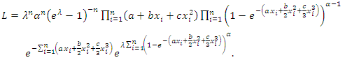
from  then the likelihood function can be written as
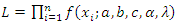 | (60) |
 | (61) |
 | (62) |
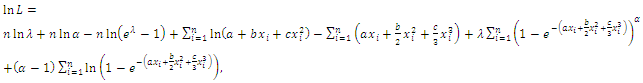
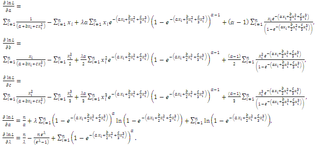 The likelihood equations can be obtained by setting the first partial derivatives of
  the unknown parameters to zero's. That is, the likelihood equations are:
 | (63) |
 | (64) |
 | (65) |
 | (66) |
 | (67) |
 | (68) |
 The normal equations do not have explicit solutions and they have to be obtained numerically. Therefore, the MLEs of
  can be obtained by solving system of three nion-linear equations with two non-linear equations.
9.2. Asymptotic Confidence Bounds
- Since the MLEs of the unknown parameters
 cannot be obtained in closed forms, it is not easy to derive the exact distributions of the MLEs. In this section, we derive the asymptotic confidence intervals of these parameters when
  The simplest large sample approach is to assume that the
  are approximately multivariate normal with mean
  and covariance matrix
  , see Lawless (2003), where
  is the inverse of the observed information matrix
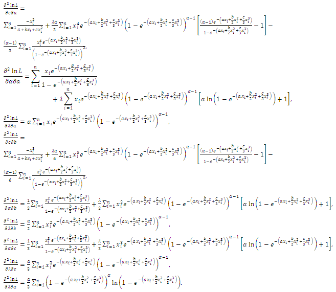
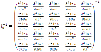 | (69) |
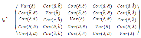 | (70) |
 are given as follows:
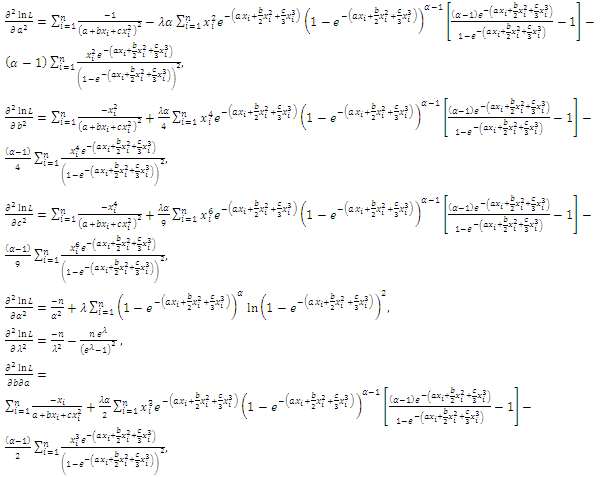
 The above approach is used to derive the
  confidence intervals of the parameters
  as in the following forms
 | (71) |
 is the upper
  percentile of the standard normal distribution. It should be mentioned here as it was pointed by a referee that if we do not make the assumption that the true parameter vector
  is an interior point of the parameter space then the asymptotic normality results will not hold. If any of the true parameter value is 0, then the asymptotic distribution of the maximum likelihood estimators is a mixture distribution, see for example Self and Liang (1987) in this connection. In that case obtaining the asymptotic confidence intervals becomes quite difficult and it is not pursued here.
10. Application
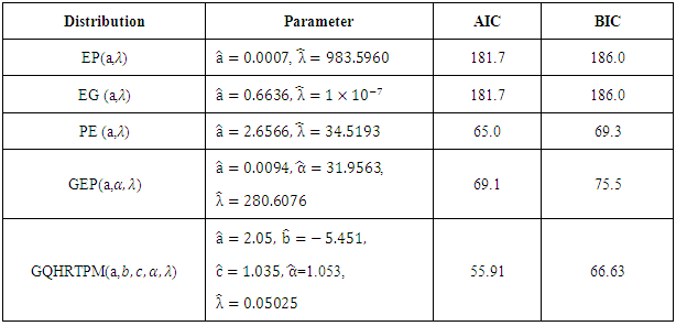
- Here, we illustrate applicability of the GQHRTPM distribution using real data sets from Smith and Naylor (1987) represents the strengths of 1.5cm glass fibres, measured at the National Physical Laboratory, England and they are taken.We compare the fit of the GQHRTPM distribution with those of the Exponential Poisson (EP), Generalized Exponential Poisson (GEP) and the Exponentiated Exponential Poisson (EEP) distributions. For each distribution, the unknown parameters are estimated by the method of maximum likelihood. The maximum likelihood estimates and the corresponding AIC and BIC values are shown in Tables 1. We can see that the smallest AIC and BIC are obtained for the GQHRTPM distribution.
|
11. Conclusions
- We introduce a new five-parameter distribution called the generalized quadratic hazard rate truncated poisson (GQHRTPM) distribution. This distribution contains several lifetime sub-models such as: EP, EG, PE and GEP. Various properties of the proposed distribution are discussed in Section 3, 4 and 5. Rényi and Shannon entropies of the GQHRTPM distribution are given in Section 6. Residual and reverse residual life functions of the GQHRTPM distribution are discussed in Section 7. Section 8 is devoted to the Bonferroni and Lorenz curves of the GQHRTPM distribution. The maximum likelihood estimation procedure is presented. Fitting the GQHRTPM model to real data set indicate the flexibility and capacity of the proposed distribution in data modeling. In view of the density and failure rate function shapes, it seems that the proposed model can be considered as a suitable candidate model in reliability analysis, biological systems, data modeling, and related fields.