1. Introduction

Data analysts are frequently faced with situations where one or several time series observations are missing at certain points within the data set collected for modeling. This creates missing values at such points. Being unable to account for missing values may result in a severe misrepresentation of the phenomenon under study or can cause havoc in the estimation and forecasting of linear and nonlinear time series as in [1]. The missing values can be reconstructed using imputation techniques. The basic idea of an imputation approach, in general, is to substitute a plausible value for a missing observation and to carry out the desired analysis on the completed data as in [2]. There are several methods that can be used for imputing missing values in numerical data. These methods include mean substitution, linear regression, neural networks and nearest neighbor approach and optimal linear interpolation.

In this study we were interested in estimating missing values for a class of bilinear nonlinear time series models called the pure bilinear time series models whose innovations have a student-t distribution using linear interpolation approach. The student-t distribution can be used to model the innovation of financial data which is known to be highly skewed. There is no evidence to show that optimal linear interpolation approach has been used to estimate missing values for bilinear time series and specifically, pure bilinear time series.

1.1. Bilinear Models

A discrete time series process is said to be a bilinear time series model of order BL (p, q, P, Q) if it satisfies the difference equation

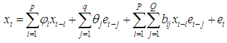(1)

where are constants; the innovation sequence are i.i.d random process which has a student-t distribution and =1. For pure bilinear time series, only the bilinear coefficient is not equal to zero. Thus the pure bilinear time series model, BL(0,0,P,Q) is given by

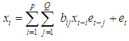(2)

where are the coefficients of the model, and are i.i.d student-t process with zero mean and common finite variance. Some important properties of this model such as invertibility and stationarity have been studied. Invertibility conditions for some particular stationary bilinear models has been derived as in [3] and [4]. [5] has established the conditions under which the general bilinear model is invertible and a condition of invertibility of model (2) can be derived from this result. This condition is expressed as

where is the correlation coefficient. The notion of invertibility is very useful for statistical applications, such as the prediction of given its past.

A stationary bilinear model can be expressed in a kind of moving average with infinite order as in [6]. This enhances its application in making inferences. Bilinear models have the property that although they involve only a finite number of parameters, they can approximate with arbitrary accuracy ‘reasonable’ nonlinearity. [7] showed that with a large bilinear coefficient b_ij, a bilinear model can have sudden large amplitude bursts and is suitable for some kind of seismological data such as earthquakes, underground nuclear explosions. The variant of the bilinear process is time dependent. This feature enables bilinear process to be used also for financial data as in [8].Researchers have achieved forecast improvement with simple nonlinear time series models. [9] reported a forecast improvement with bilinear models in forecasting stock prices. The statistical properties of such models have been analyzed in detail as in [4], [10], [11] and [12].

Several techniques have been used in estimating missing values. Most of them are nonparametric and includes use of artificial neural network as in [13]; [14]; [15] and exponential smoothing as in [16]. The techniques used for estimating missing values do not consider the distribution of the innovation sequence. They also don not consider nonlinear models. Therefore in this study estimates of missing values for nonlinear bilinear time series models with student-t distribution are derived using an optimal linear interpolation technique based on minimizing the h-steps-ahead dispersion error.

2. Literature Review

2.1. Student-t Distributions

The departure from the standard white noise is becoming prevalent in the literature of nonlinear time series as in [17]. An alternative distribution that can be used is the student-t distribution. It plays an important role in modeling. [18] presents the R package BayesGach which provides functions for the Bayesian estimation of the parsimonious and effectiveGarch (1,1) model, with student-t innovations. The Garch (1,1) model with student-t distribution is able to reproduce the volatility dynamism of financial data. Given a model, specification for log of return disturbances can be modeled using either the student-t distribution or the normal distribution. The student-t is particularly useful since it can provide the excess kurtosis in the conditional distribution that is found in financial time series unlike the models with normal innovations.

[19] focused on the bilinear time series model with GARCH innovations (BL-GARCH). It has an important property that it can take into account explosions and related volatility features of non-linear time series. Specifically, he studied the BL-GARCH (1,1) process, which is mainly used in applications with normal, Student-t and GED noises. Other than the normal (stable) case the distribution of the white noise {e_t} is often quite different from that of the observations X_t. [20] have shown that X_t and {e_t} both can have student-t distribution if the noise is allowed to be non-white (exchangeable).

2.2. Missing Value Imputation: Linear Time Series Models with Finite Variance

[21] discussed a method based on forecasting techniques to estimate missing observations in time series. He also compared this method with other methods using minimum mean square estimate as a measure of efficiency based on forecasting techniques. [22] obtained estimates of missing values for time series processes with finite variance.

Within the frame work of the state space formulation, estimates of missing values and their corresponding error variance can be derived conveniently through the use of recursive smoothing methods associated with Kalman filter. Such smoothing methods are described in general terms as in [23]. Algorithms for computing the likelihood function when there are missing data in scalar case have been provided by [24] and [25]. They also showed how to predict and interpolate missing observations and obtain the mean squared error of the estimate. [25] pointed out that the problem can be solved by setting up the model in state space form and applying the Kalman filter.

[1] Applied both the kalman filter and optimal linear estimation method and demonstrated the superiority of the optimal method. [26] used kalman filter to estimate missing values for AR(1) model. They withheld values at certain points and then estimated them as though they were missing. Their results revealed that simple exposition of state space representation for commonly used time series models can be formulated.

[27] developed an optimal method that is based on linear combination of the forward and back forecasts for estimating missing values for ARMA time series models. [28] discussed different alternatives for the estimation of missing observation in stationary time series for autoregressive moving average models. [29] demonstrated that missing values in time series can be treated as unknown parameters and estimated by maximum likelihood or as random variables and predicted by the expectation of the unknown values given the data. [10] extended the concept of using minimum mean square error linear interpolator for missing values in time series to handle any pattern of non-consecutive observations. The paper refers to the application of simple ARMA models in discussing the usefulness of either the nonparametric or the parametric form of the least squares interpolator.

Later, [30] demonstrated a linear recursive technique that does not use the Kalman filter to estimate missing observations in univariate time series. It is assumed that the series follows an invertible ARIMA model. This procedure is based on the restricted forecasting approach, and the recursive linear estimators are obtained when the minimum mean-square error are optimal. It is evident that Kalman filter technique has been widely used as an imputation method for ARMA processes.

2.3. Missing Value Imputation: Nonlinear Time Series Models

[31] derived a recursive estimation procedure based on optimal estimating function and applied it to estimate model parameters to the case where there are missing observations as well as handle time-varying parameters for a given nonlinear multi-parameter model. More specifically, to estimate missing observations,they formulated a nonlinear time series model which encompasses several standard nonlinear models of time series as special cases. It also offers two methods for estimating missing observations based on prediction algorithm and fixed point smoothing algorithm as well as estimating functions equations. However, little was done on bilinear time series models.

[32] investigated influence of missing values on the prediction of a stationary time series process by applying Kaman filter fixed point smoothing algorithm. He developed simple bounds for the prediction error variance and asymptotic behavior for short and long memory process.

[33] derived a recursive form of the exponentially smoothed estimated for a nonlinear model with irregularly observed data and discussed its asymptotic properties. They made numerical comparison between the resulting estimates and other smoothed estimates. It is evident that not much has been done on missing value estimation for bilinear time series models.

2.4. Classes of Bilinear Models Studied

The bilinear model has been widely applied in many areas such as control theory, economics and finance. The structure of model (1) has been studied in the literature especially for some special cases. For example, [7] considered model BL (p,o,p,q); [11] studied the asymptotic behaviour of the correlation function for the simple bilinear model BL(0,0,1,1); [34], [35] and [36] studied the model BL(1,0,1,1); [37] considered the model BL(0,0,1,1). [38] estimated the coefficients of a bilinear model using the maximum likelihood method. However, she restricted the analysis to investigating the subclass of bilinear processes with a single bilinear term, BL(1, 0, 1, 1).

[39] claimed that estimating bilinear models is quite challenging. Many different ideas have been proposed to solve this problem. However, there is not a simple way to do inference even for its simple cases. They proposed a generalized autoregressive conditional heteroskedasticity - type maximum likelihood estimator for estimating the unknown parameters for a special bilinear model.

It can be seen from the literature that there are a variety of methods used for estimating missing values for different time series data. What is however lacking is an explicit method for estimating missing values for bilinear time series models. We therefore want to estimate missing values for bilinear time series which have different probability distributions.

2.5. Estimation of Missing Values Using Linear Interpolation Method

Suppose we have one value missing out of a set of an arbitrarily large number of n possible observations generated from a time series process . Let the subspace be the allowable space of estimators of based on the observed values i.e., where n, the sample size, is assumed large. The projection of onto (denoted ) such that the dispersion error of the estimate (written disp is a minimum would simply be a minimum dispersion linear interpolator. Direct computation of the projection onto is complicated since the subspaces and are not independent of each other. We thus consider evaluating the projection onto two disjoint subspaces of To achieve this, we express as a direct sum of the subspaces and another subspace, say such that. A possible subspace is, where is based on the values . The existence of the subspaces is shown in the following lemma.

2.5.1. Lemma

Suppose is a nondeterministic stationary process defined on the probability space . Then the subspaces defined in the norm of the are such that

Proof:

Suppose can be represented as

where . Clearly the two components on the right hand side of the equality are disjoint and independent and hence the result. The best linear estimator of can be evaluated as the projection onto the subspaces and such that disp is minimized. i.e.,

But

where the coefficients’ are estimated such that the dispersion error is minimized. The resulting error of the estimate is evaluated as

Now squaring both sides and taking expectations, we obtain the dispersion error as

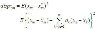(1)

By minimizing the dispersion with respect to the coefficients (differentiating with respect to and solving for ) we should obtain the coefficients 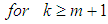which are used in estimating the missing value. The missing value is estimated as

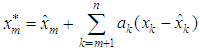(2)

3. Research Methodology

The data was simulated from pure bilinear time series models: BL(0,0,1,1) and BL(0,0,2,1) which have student-t innovations using R-statistical software. For each bilinear time series model, a program code was used to simulate the data. 100 samples of size 500 were generated and missing artificial points were created at data point 48, 293 and 496. These points were selected at random. Data analysis was done using statistical and computer software which included Excel, TSM and R and Matlab7. The mean square error (MSE) and mean absolute deviation (MAD) were used as performance measures. The MAD (Mean Absolute Deviation) and MSE (Mean Squared Error) were used. These were obtained from equation (3) and equation (4) respectively.

4. Results

4.1. Derivation of the Missing Values for Bilinear Time Series Models with Student-t Innovations

Estimates of missing values for pure bilinear time series models whose innovations follow student-t distributions were derived based on minimizing the h-steps-ahead dispersion error. Two assumptions were made in the process of the derivations. The first one was that the time series data is stationary and thus their roots lie within the unit circle. Secondly, the higher powers (of orders greater than two or products of coefficients of orders greater than two) of the coefficients are approximately negligible. This was consequence of the result of the first assumption. Recall from lemma 2.12 and equations (1) that the optimal linear estimate for the missing observation is by given 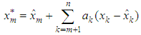where is the estimate obtained from the model based on the previous lagged observations of the data before the point m, the missing data point and x_m the missing value, the coefficients are to be estimated by minimizing the dispersion error given by equation (1).

4.2. Estimates of Missing Values BL (0,0,1,1) with Student T Errors

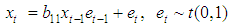
The pure bilinear time series model with student t innovations of order one BL (0, 0, 1,1) is of the form

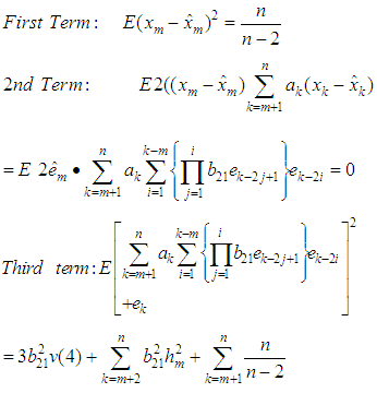
The estimate of the missing value for this model is given by theorem 4.1.

Theorem 4.1

The optimal linear estimate for missing observation for BL (0, 0, 1,1) with student errors is given by

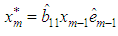Proof

The stationary bilinear model, BL (0, 0, 1,1) is given by

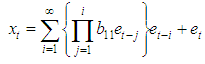and the h-steps ahead forecast is

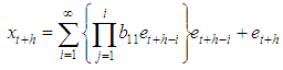Therefore the forecast error is

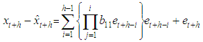(5)

Substituting equation (5) in equation (1) we have,

(6)

Simplifying each of the terms of equation (6), we obtain the following:

Hence equation (6) can be simplified as

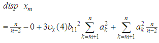Now differentiating equation (4) with respect to and equating to zero, we obtain\

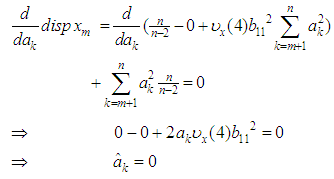Substituting the values of in equation (1), we obtain best estimator of the missing value as

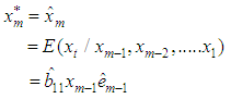This shows that the missing value is a one-step-ahead forecast based on the past observations collected before the missing value. This is in agreement with other studies that have estimated missing values using forecasting as in [29] and [1].

Theorem 4.2

The optimal linear estimate for BL (0,0,2,1) with student–t distribution

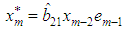Proof

The stationary BL(0,0,2,1) is given by

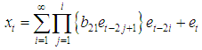The h-steps ahead forecast error is expressed as

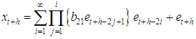Therefore the forecast error is

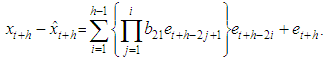or it can also be represented as

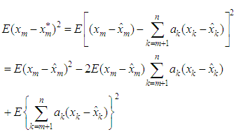
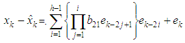Substituting equation (6) in equation (1), we have

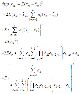(9)

Simplifying each term of equation (9) separately, we have

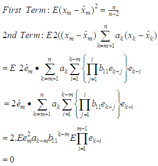
Hence equation (7) can be simplified as

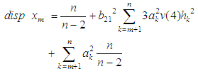(10)

Now differentiating equation (10) with respect to and equating to zero, we obtain

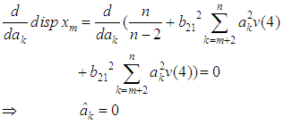Therefore the estimate of the missing value for the BL(0,0,2,1) is

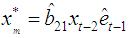
4.3. Simulation Results

In this section, the results of the optimal linear estimate, artificial neural networks and exponential smoothing based on simulated generated data for the student-t distributed innovations are presented. The R software was used to generate the bilinear random variables. One hundred samples of size 500 were generated for each model and missing values created at positions 48, 293 and 496. The mean absolute deviation and mean square deviations were calculated for each model used. The data generated were plotted in Figure 1-2 below.

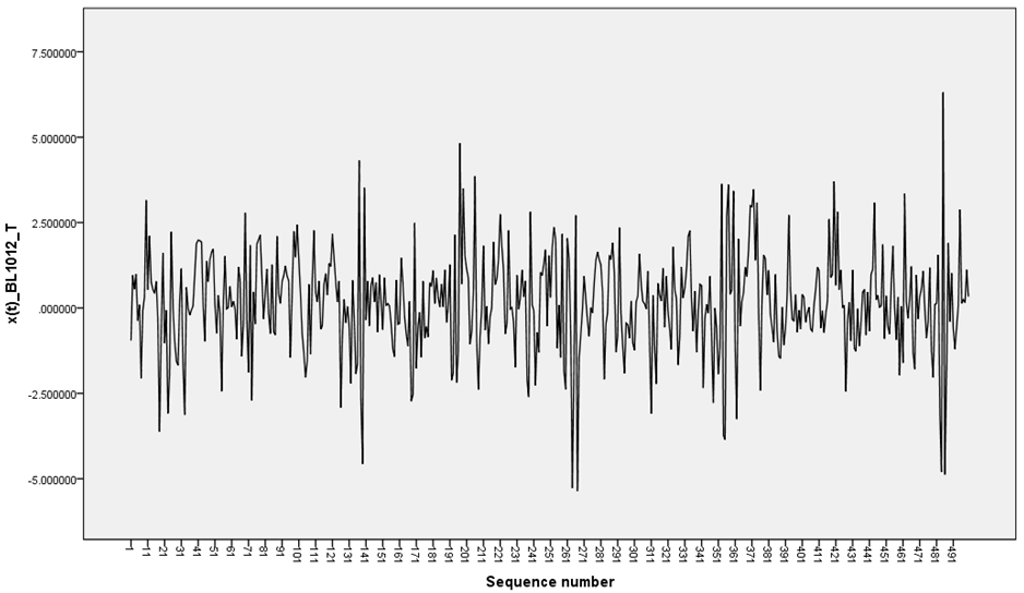Figure 1. BL(0,0,1,1) with t-distributed innovations

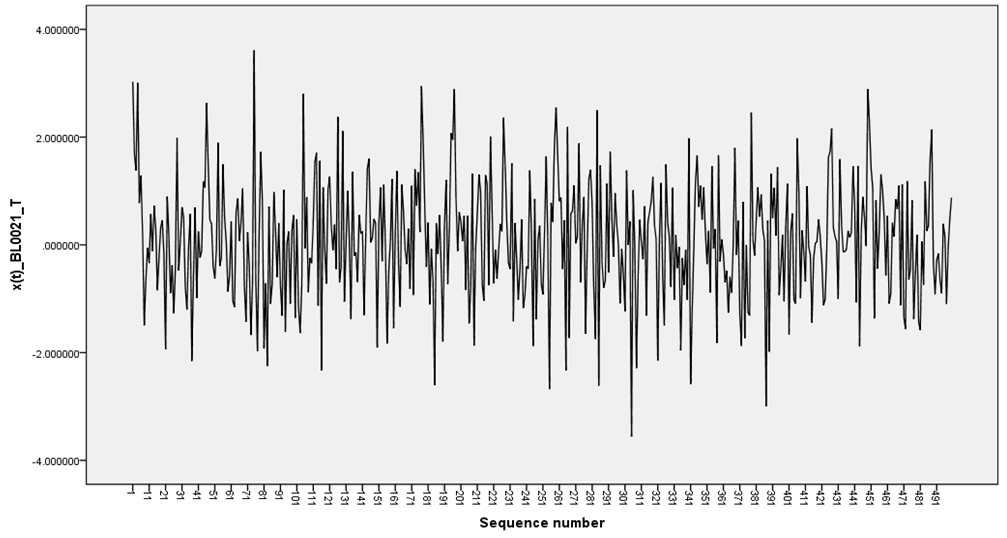Figure 2. BL(0,0,2,1).with t-istributed innovations

These graphs are characterized by sharp outburst. Sharp outburst is one of the characteristics of nonlinearity in bilinear models. For Bilinear time series with student-t distributions, the range of the values is also large. The results of the efficiency of the estimates are given in table given in tables 1-2.

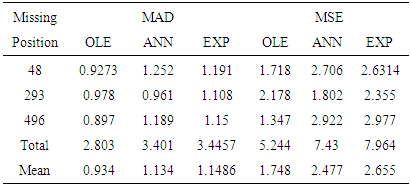Table 1. Efficiency Measures obtained for student-tBL (0,0,1,1)

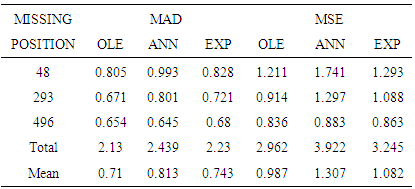Table 2. Efficiency Measures obtained for student-BL(0,0,2,1)

From table 1, it can be concluded that based on MAD, the OLE estimates of missing values were the most efficient (overall mean MAD=0.934 for the different missing data point positions followed by ANN estimates (overall mean MAD=1.134).

From table 2, it can be concluded that based on MAD, the OLE estimates of missing values were the most efficient (overall mean MAD=0.71) for the different missing data point positions followed by EXP smoothing estimates (overall mean MAD=0.813). It is also evident that the size of the set of values used to estimate the missing values had a positive correlation with the efficiency of the estimates obtained for all the estimators. All estimates for data at position 48 were less efficient than estimates obtained at data points 293 and 496. The estimates became more efficient as the position of missing data increased.

5. Conclusions

In this study we have derived estimates for missing values for pure bilinear time series with student-t innovations. The missing values were found to be equivalent to the one–step-ahead forecast based on the lagged observations before the point of the missing value. Therefore to estimate missing values for pure bilinear time series which has student t distribution, we use one step ahead forecast. Further, the study found that the efficiency of the estimates obtained are correlated with the position of the missing observation. The further the position of the missing value from the first observation, the less efficient the estimate is. The estimates based on linear interpolation were on average better than the estimates based on ANN and exponential smoothing.

6. Recommendations

The study recommends that for bilinear time series data with student t-innovations, OLE estimates be used in estimating missing values. More research needs to be done on whether the accuracy of an imputation method depends on the distribution of the data. Other research should focus on the comparison of the efficiency of the estimates obtained using other techniques such as kalman filter and estimation function. Other distributions for the innovation sequence should be considered.

Appendix

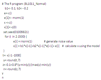
This appendix has two parts, Appendix A and B. Appendix A contains the R codes used in simulating the time series data used in the analysis. The same codes are also used to obtain normalized data used in artificial neural network imputations. The moments of the various distributions are given in Appendix B. The codes for different bilinear models used in this data are given below.

Appendix A. Program Codes used in simulation