Maxwell A. Boateng, A. Y. Omari-Sasu, Nana K. Frempong
Mathematics Department, Kwame Nkrumah University of Science and Technology, Kumasi, Ghana
Correspondence to: Maxwell A. Boateng, Mathematics Department, Kwame Nkrumah University of Science and Technology, Kumasi, Ghana.
| Email: |  |
Copyright © 2015 Scientific & Academic Publishing. All Rights Reserved.
This work is licensed under the Creative Commons Attribution International License (CC BY).
http://creativecommons.org/licenses/by/4.0/

Abstract
The study investigated the presence of volatility in two insurance companies listed on the Ghana Stock Exchange. In checking for the presence of volatility, several ARIMA (p,d,q) models were fitted separately to the log return series of the two companies and the best model selected using the AIC and BIC selection criterion. Using the selected ARIMA (p,d,q) models, the residuals of the model were obtained and presence of ARCH effects evaluated using the ARCH-LM test for each company. The ARCH-LM test revealed that there were no ARCH effects in both companies, thus, fitting either an ARCH or a GARCH model to the series was not the best. The ARIMA (1,0,2) model was thus used in forecasting the returns of EGL whereas the ARIMA (1,0,1) model was used in forecasting returns of SIC.
Keywords:
Volatility, Heteroscedasticity, Log returns, Stationarity, ARCH effects, GARCH
Cite this paper: Maxwell A. Boateng, A. Y. Omari-Sasu, Nana K. Frempong, Volatility Assessment of Equities on the Ghana Stock Exchange, International Journal of Statistics and Applications, Vol. 5 No. 6, 2015, pp. 288-292. doi: 10.5923/j.statistics.20150506.04.
1. Introduction
The very existence of man has been confronted with making choices. In business, in agriculture, in the industry, etc., man is presented with the problem of selecting one possibility over the other. Usually, businesses, individuals companies and government agencies forecast increase in demand and need to raise additional capital to meet their needs. An accurate measurement of forecast of expected future events is not easy to assert since most activities have uncertain future or outcome. There is therefore risk in everything we do. Risk is a fact of life and for any investor risk must be considered in every financial decision making. When investors put up their money to buy shares of a company at the stock market, they expect to receive returns on their investment from future cash flows otherwise they would not invest. However, there is a potential variability to such future cash flows. There is also the possibility that the sales of a company may decline relative to its past sales or the company may be bankruptcy and collapse. In such an uncertainty occupied world, an accurate measurement of expected future cash flows is not easy for an investor to ascertain. It is therefore necessary to assess volatility and its effect on returns.
2. Related Works
Andrei and Hasler (2015) investigated the joint role played by investors' attention to news and learning uncertainty in determining asset prices in a theoretical framework. Their model provided two main predictions. The first was that stock return variance and risk premia increased with both attention and uncertainty. The second prediction was that the increasing relationship was quadratic. They tested the two predictions and showed that the data gave support to the increasing relationship. The evidence for a quadratic relationship however, was mixed. Their study showed theoretically and empirically that both attention and uncertainty are key determinants of asset prices.King and Wadhwani (1990) investigated why, in October 1987, almost all stock markets fell together despite widely differing economic circumstances. They constructed a model in which contagion between markets occured as a result of attempts by rational agents to infer information from price changes in other markets. Their model provided a channel through which a mistake in one market could be transmitted to other markets.According to Shiller, If the volatility of stock market prices was to be understood in terms of the efficient markets hypothesis, then there had to be evidence that true investment value changed through time sufficiently to justify the price changes. He considered three indicators of change in true investment value of the aggregate stock market in the United States from 1871 to 1986; changes in dividends, in real interest rates, and in a direct measure of inter-temporal marginal rates of substitution. Although there were some ambiguities in interpreting the evidence, dividend changes appeared to contribute very little toward justifying the observed historical volatility of stock prices. The other indicators contributed some. Most of the volatility of stock market prices appeared unexplained however.Hamao et. al (1990) examined the short-run interdependence of prices and price volatility across three major international stock markets using daily opening and closing prices of major stock indexes for the Tokyo, London, and New York stock markets. Their analysis utilized the autoregressive conditional heteroscedastic (ARCH) family of statistical models to explore these pricing relationships. Ivo et. al (2008) provided empirical evidence on the link between stock market volatility and macroeconomic uncertainty. They showed that US stock market volatility was significantly related to the dispersion in economic forecasts from participants in the Survey of Professional Forecasters over the period 1969 to 1996. The relationship was much stronger than that between stock market volatility and the more traditional time-series measures of macroeconomic volatility, but disappeared from 1997 onwards. This coincided with a previously documented regime shift in stock volatility. Nagajara and Naresh (2013) worked in the field of Indian share markets taking into account one year data from January 2010 to December 2010. Their research included how the share prices of various selected companies varied with respect to economic factors. Their research work included the collection of data regarding the share prices of the selected companies during one year and the SENSEX. Their research attempted to study the relationship of stock returns with macroeconomic variables in Indian context. The data consisted of 12 months from January 2010 to December 2010 comprising of two macro indicators (Exchange Rate & inflation rate) for the study.Marco et. al (1999) studied the volatility of the MIB30-stock-index high-frequency data from November 28, 1994 through September 15, 1995. Their study was aimed at empirically characterizing the volatility random walk in the framework of continuous-time finance. They computed the index volatility by means of the log-return standard deviation choosing an hourly time window in order to investigate intraday properties of volatility. They found a periodic component for the hourly time window, in agreement with previous observations. Fluctuations were studied by means of detrended fluctuation analysis and long-range correlations were detected. Volatility values were found to be log-stable distributed. Adams et. al (2012) provided a user-friendly approach to explain how variation in fundamental price-determining variables translated into variation in the fundamental value of equities, based on the standard dividend-growth model. Their analysis wa illustrated with UK data using estimates of real interest rate forecasts and real dividend growth rate forecasts in the past. Their work showed that actual market volatility did not appear to be excessive when compared with the notional volatility implied by changes over.
3. Methodology
The study uses time series techniques such as; Box-Jenkins model (ARIMA) and ARCH/GARCH model to investigate market volatility of two insurance companies. Data for the study was obtained from the Ghana Stock Exchange website (www.gse.com.gh). The R software is used for the analysis. The closing prices of each company was obtained for the duration under study and transformed using the log return (continuously compounded return). The general form of the ARIMA (p,d,q) model is given as: | (1) |
Where, are polynomials in terms of B of degree p and q and B is the backward shift operator.
 are the autoregressive parameters with order p
 are the moving average parameters with order qThe continuously compounded return or log return is the natural logarithm of the simple gross return of an asset.
 | (2) |
Continuously compounded returns  have some advantages over the simple net returns
  . Considering multi-period returns;
 | (3) |
The ARCH LM test is equivalent to the usual F-statistic for testing  in the linear regression
  | (4) |
Where,  denotes the error termm is a prespecified positive integer T is the sample sizeThe null and alternative hypotheses are;
4. Results
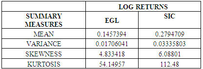
The study uses the daily log returns (continuously compounded returns) of two (2) listed companies, which are Enterprise Group Limited (EGL) and State Insurance Company (SIC) from the year 2008 to 2014. The daily return series for each of the companies was obtained and transformed accordingly.Table 1 gives some descriptive statistics of the log return series of both EGL and SIC. SIC is seen to have the highest log return (0.2794709) with that of EGL being 0.1457394. Table 1. Descriptive Statistics of Daily Log Returns of EGL and SIC
 |
| |
|
4.1. Process for Volatility
From Tsay (2005), fitting a volatility model for an asset return series takes the following steps:i. Specifying a mean equation by testing for serial dependence in the data and, if necessary, building an econometric model (e.g., an ARMA model) for the return series to remove any linear dependence.ii. Using the residuals of the mean equation to test for ARCH effects.iii. Specifying a volatility model if ARCH effects are statistically significant and perform a joint estimation of the mean and volatility equations.iv. Checking the fitted model carefully and refine it if necessary.
4.1.1. Test for Stationarity EGL
Using the KPSS Test for Level Stationarity with the hypotheses below:Ho: level stationaryHa: not stationaryWith a p-value of 0.01, the null hypothesis of level stationarity for the KPSS test was rejected. This implied that the series was not stationary. After differencing once, the series stationarity was achieved.
4.2. ARIMA Model Evaluation for Log Return Series of EGL
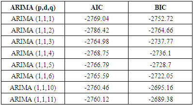
Based on the ACF and PACF plots of the first differenced series, several ARIMA (p,d,q) models were fitted to the log return series of EGL. Table 2 below is a summary of the models.Table 2. ARIMA (p,d,q) with AIC and BIC
 |
| |
|
From table 2 above, the model with smallest AIC and BIC was the ARIMA (1,1,2) model, thus it is the selected model.
4.3. ARIMA (1,1,2) Model
 sigma^2 estimated as 0.01136: log likelihood=1397.21AIC=-2786.42
  AICc=-2786.4
  BIC=-2764.66Thus, the full ARIMA (1,1,2) is given as;
4.4. ARCH LM Test for Heteroscedasticity of EGL Series
In order to apply an ARCH/GARCH model or any of its variants to a series, the residuals of that series need to be tested for conditional heteroscedasticity. The ARCH Lagrange Multiplier (ARCH LM) test is employed for this process.Table 3. ARCH Test with Degrees Of Freedom and P-Values
 |
| |
|
Table 3 above shows that the residual series of EGL exhibited no ARCH effects, implying that the series are homoscedastic. Thus, the ARIMA (1,1,2) is adequate enough to represent the log return series of EGL. The ARCH/GARCH models are therefore not required for this series.
4.5. Test for Stationarity SIC
Using the KPSS Test for Level Stationarity with the hypotheses below:Ho: level stationaryHa: not stationaryWith a p-value of 0.1, the null hypothesis of level stationarity for the KPSS test was not rejected. This implied that the series was stationary, hence no differencing was required.
4.6. ARIMA Model Evaluation for Log Return Series of SIC
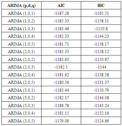
Based on the ACF and PACF plots of the log return series of SIC, several ARIMA (p,d,q) models are fitted to the series and the on with the smallest AIC and BIC selected. From table 4, the model with the smallest AIC and BIC is ARIMA (1,0,1).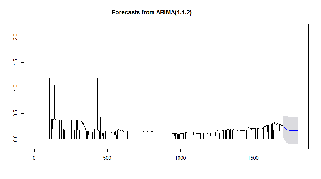 | Figure 1. Plot of forecast for 100 days ahead for the EGL series |
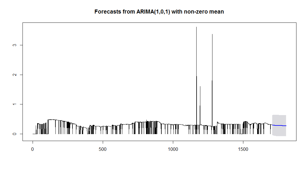 | Figure 2. Plot of forecast for 100 days ahead for the EGL series |
Table 4. ARIMA (p,d,q) with AIC and BIC
 |
| |
|
4.7. ARIMA (1,0,1) Model
 sigma^2 estimated as 0.02906: log likelihood=597.64AIC=-1187.28
  AICc=-1187.26
  BIC=-1165.51Thus, the full ARIMA (1,0,1) is given as;
4.8. ARCH LM Test for Heteroscedasticity of SIC Series
In order to apply an ARCH/GARCH model or any of its variants to a series, the residuals of that series need to be tested for conditional heteroscedasticity. The ARCH Lagrange Multiplier (ARCH LM) test is employed for this process.Table 5. ARCH Test with Degrees Of Freedom and P-Values
 |
| |
|
Table 5 above shows that the residual series of SIC exhibited no ARCH effects, implying that the series are homoscedastic. Thus, the ARIMA (1,0,1) model is adequate enough to represent the log return series of SIC. The ARCH/GARCH models are therefore not required for this series.
5. Conclusions
The study investigated the presence of volatility in two insurance companies The process of modelling volatility involves fitting an ARIMA (p,d,q) model, obtaining the residuals of the said model and testing for ARCH effects on the residuals. If the residual series exhibit ARCH effects, then ARCH/GARCH models can be considered.The returns series of these two companies were obtained and each of them was tested for stationarity using the KPSS test. The series for EGL were found to be non-stationary, thus, a first difference was applied to the series and stationarity was achieved. Based on the ACF and PACF plots of the differenced EGL series, several ARIMA (p,d,q) models were fitted to the series. The model that performed best was found to be ARIMA (1,1,2). The residuals of the ARIMA (1,1,2) model were obtained in subjected to the ARCH-LM test for conditional heteroscedasticity. Using lags 5, 12, 18and 20, the series were found to have constant variance (thus, heteroscedasticity not present). Since there were no ARCH effects, there was no need to fit an ARCH/GARCH model or any of its variants. The ARIMA (1,1,2) was thus adequately sufficient for prediction.Analysing the SIC log return series, it was found to be stationary by the KPSS test. An assessment of the ACF and PACF plots led to fitting several ARIMA (p,d,q) models. Among those models, the ARIMA (1,0,1) model was found to have the least AIC as well as BIC. Residuals of the model were obtained and tested for conditional heteroscedasticity. Once again, the residual series were found to have no ARCH effects. Thus, an ARCH/GARCH or any of its variants were not needed. In conclusion, the two models for the companies were all ARIMA (p,d,q) models and they were adequate for forecasting according to the study.We wish to thank the National Institute for Mathematical Sciences (NIMS) Ghana for supporting this study.
References
| [1] | Daniel Andrei, Michael Hasler, “Investor Attention and Stock Market Volatility”, Rev. Financ. Stud. (2015) 28 (1): 33-72. doi: 10.1093/rfs/hhu059. |
| [2] | Mervyn A. King and Sushil Wadhwani, “Transmission of Volatility between Stock Markets”, Rev. Financ. Stud. (1990) 3 (1): 5-33. doi: 10.1093/rfs/3.1.5. |
| [3] | Robert J. Shiller, “The Volatility of Stock Market Prices”, Science 2 January 1987, Vol. 235 no. 4784 pp. 33-37, DOI:10.1126/science.235.4784.33. |
| [4] | Yasushi Hamao, Ronald W. Masulis, Victor Ng, “Correlations in Price Changes and Volatility across International Stock Markets”, Rev. Financ. Stud. (1990) 3 (2): 281-307. doi: 10.1093/rfs/3.2.281. |
| [5] | Ivo J. M. Arnold, Evert B. Vrugt, “Applied Financial Economics, Volume 18, Issue 17, 2008, pages 1425-1440, DOI:10.1080/09603100701857922. |
| [6] | Nagaraja, P.; Naresh, Ch. (2013), “A Study On Volatility Of Share Prices With Respect To Economic Factors”, Asia Pacific Journal Of Research In Business Management; Mar2013, Vol. 4 Issue 3, P1. |
| [7] | Marco Raberto, Enrico Scalas, Gianaurelio Cuniberti, Massimo Riani, “Volatility in the Italian Stock Market: an Empirical Study”, Physica A 269, 148-155 (1999), DOI:10.1016/S0378-4371(99)00089-8. |
| [8] | Andrew Adams, Seth Armitage, Adrian FitzGerald, “An analysis of stock market volatility”, Annals of Actuarial Science, Volume 6, Issue 01, March 2012, pp 153-170, DOI: http://dx.doi.org/10.1017/S1748499511000339. |
| [9] | Tsay, R. S. (2005). Analysis of Financial Time Series. John Wiley & Sons, Inc., Hoboken, New Jersey, 2nd Ed. |


 are polynomials in terms of B of degree p and q and B is the backward shift operator.
 are the autoregressive parameters with order p
 are the moving average parameters with order qThe continuously compounded return or log return is the natural logarithm of the simple gross return of an asset.
 have some advantages over the simple net returns
  . Considering multi-period returns;
 in the linear regression
 denotes the error termm is a prespecified positive integer T is the sample sizeThe null and alternative hypotheses are;
 sigma^2 estimated as 0.01136: log likelihood=1397.21AIC=-2786.42
  AICc=-2786.4
  BIC=-2764.66Thus, the full ARIMA (1,1,2) is given as;


 sigma^2 estimated as 0.02906: log likelihood=597.64AIC=-1187.28
  AICc=-1187.26
  BIC=-1165.51Thus, the full ARIMA (1,0,1) is given as;
 Abstract
 Reference
 Full-Text PDF
 Full-text HTML