Ronald W. Wanyonyi1, Kennedy L. Nyongesa2, Adu Wasike2
1Department of Mathematics, Egerton University, Nakuru, Kenya
2Department of Mathematics, Masinde Muliro University of Science and Technology, Kakamega, Kenya
Correspondence to: Ronald W. Wanyonyi, Department of Mathematics, Egerton University, Nakuru, Kenya.
| Email: |  |
Copyright © 2015 Scientific & Academic Publishing. All Rights Reserved.
This work is licensed under the Creative Commons Attribution International License (CC BY).
http://creativecommons.org/licenses/by/4.0/

Abstract
Batch testing has long been recognized as an efficient method of classifying all the experimental units into two mutually exclusive categories: defective or non-defective. In recent years, more focus has been on estimation of the population proportion p of a trait of interest using batch testing. However, in most of the applications, the tests used are prone to errors leading to misclassifications even though misclassifications are kept at a minimal. In this paper, an estimator of the unknown proportion of a trait using batch testing model based on a quality control process in the presence of inspection errors is constructed and its properties discussed. In quality control, a batch is rejected if the constituent defective members are greater than l, the cut off value. The proposed model is superior to the existing models when the proportion of a trait is relatively high with fixed sensitivity and specificity.
Keywords:
Quality control, Batching testing, Misclassifications, Cut off value, Proportion, Imperfect tests, Sensitivity, Specificity
Cite this paper: Ronald W. Wanyonyi, Kennedy L. Nyongesa, Adu Wasike, Estimation of Proportion of a Trait by Batch Testing with Errors in Inspection in a Quality Control Process, International Journal of Statistics and Applications, Vol. 5 No. 6, 2015, pp. 268-278. doi: 10.5923/j.statistics.20150506.02.
1. Introduction
In many applications, items can be classified as defective or non-defective. Batch testing, also known as group testing, involves pooling such items into batches and then testing the batches rather than individual items. A batch is declared non-defective if all its items do not possess the trait of interest. Batch testing has been shown to be cost and time effective when the trait of interest is rare. Batch testing has a rich history going back to Dorfman (1943) and since his seminal work; batch testing has been applied to problems in blood bank screening, genetics, drug discovery, epidemiology and quality control (see e.g Gastwirth, 2000; Remlinger et al., 2006; Hughes-Oliver, 2006, Biggerstaff, 2008; Bilder et al., 2010). In all these applications, batch testing has two main objectives; first is the identification of positive individuals in a large population (Dorfman, 1943, Johnson et. al., 1991, and Nyongesa, 2004). Second is estimation of the proportion of character or trait of interest (Thomson, 1962, Sobel and Elashoff, 1975, Garstwirth and Johnson, 1994, Brookmeyer, 1999, Hughes-Oliver and Swallow, 1994, Tu et. al., 1995 and Xie et. al., 2001).Recent studies in batch testing have concentrated on the second objective by generalizing Thomson (1962) and Sobel and Elashoff (1975) studies. The various scholars have done this by considering; unequal pool sizes (Brookmeyer, 1999, Hepworth, 1999 and Biggerstaff, 2008), multistage pooling schemes (Brookmeyer, 1999, Hughes-Oliver and Swallow, 1994 and Nyongesa, 2004) and imperfect tests (Tu et. al., 1995 and Nyongesa, 2012). But, in quality control processes a batch is classified positive or negative according to whether d, the number of constituent members with quality characteristic is greater or less than a fixed cut off value or threshold (Montegomery, 2009). This is similar to threshold batch testing introduced by Damaschke (2006) where he considered two thresholds, l < u, called the lower and upper threshold respectively. Several others authors have also considered the threshold batch testing among them are Chen and De Bonis (2011). However, they were mainly concerned with coming up with algorithms that can be used to determine the minimum number of tests required to determine the defective items. Tu et. al. (1995) described the use of batch testing in HIV surveillance and implemented the possibility of testing errors in the process. Two terms are commonly used when discussing the perfection or imperfection of a test: sensitivity and specificity. Sensitivity is the probability of a positive result given that the unit tested is truly positive. Specificity is the probability of a negative result given that the unit tested is actually negative. In this paper we present the maximum likelihood estimator for the proportion of detective, p and its properties when using batch testing in the presence of the test errors in a quality control process. That is, there is possibility of misclassification of defective or non-defective item being declared non-defective or defective respectively.
2. Estimator of Proportion
Suppose we have a set of items that can be characterized as defective or non defective and that the probability, p of being defective is same for all items in the population. Further, assume that the items can be subdivided into n batches each of size, k. Then the batches are tested with kits that are not 100% perfect. The objective is to estimate the proportion of defectiveness that characterizes the population under investigation by testing a batch. If a batch is labeled defective, then the number of constituent items with the quality character of interest, d is greater than a predetermined cut off value l. Given that  and
and  are sensitivity and specificity of the test, then the probability of classifying a batch as positive;
 | (1) |
where  | (2) |
We investigate the relationship between  and
and  by plotting
  against
  for different k and l. The value of sensitivity and specificity is fixed and assumed equal in the course of testing. Figure 1 shows the relationship between
  versus
  given that the sensitivity and specificity are equal to 99%. It can be noted that the probability increases rapidly for low p converging to the value of sensitivity.
 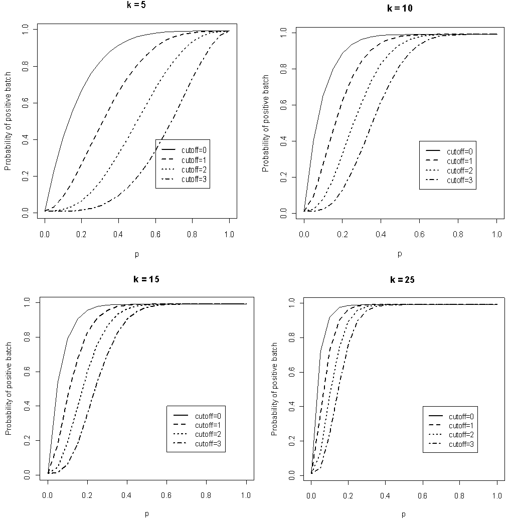 | Figure 1. Plot of  as a function of as a function of  for k = 5, 10, 15, 25 and l = 0, 1, 2, 3 with sensitivity and specificity = 99% for k = 5, 10, 15, 25 and l = 0, 1, 2, 3 with sensitivity and specificity = 99% |
Next, the value of sensitivity and specificity is fixed at 90% and the relationship observed as shown in Figure 2.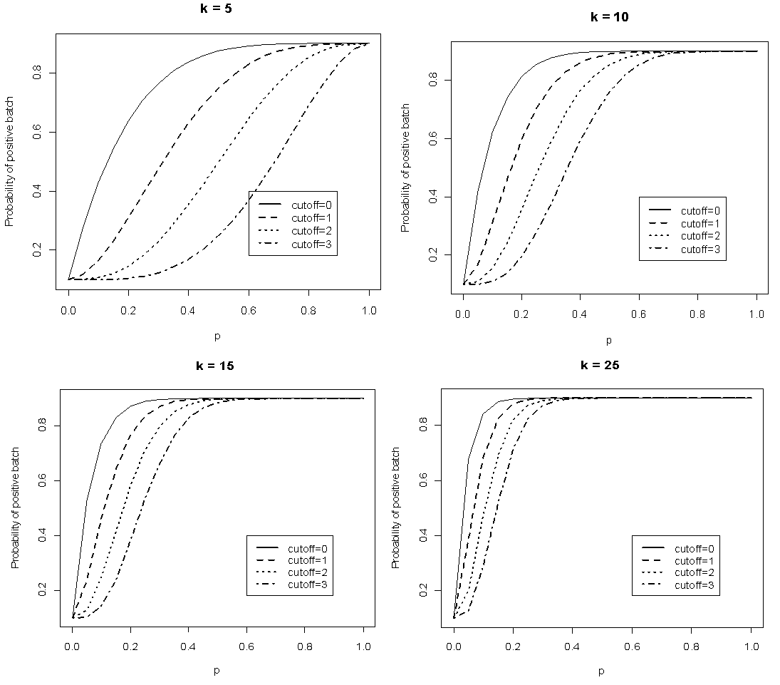 | Figure 2. Plot of  as a function of as a function of  for k = 5, 10, 15, 25 and l = 0, 1, 2, 3 with sensitivity and specificity = 90% for k = 5, 10, 15, 25 and l = 0, 1, 2, 3 with sensitivity and specificity = 90% |
The observation of Figure 2 illustrates that the relationship is monotonically increasing and the increment is steep for low values of p. The relationship was also examined for sensitivity and specificity fixed at a low value equal to 70%. This value is picked for the sole purpose of studying the relationship. This is because the tests which are normally used have higher sensitivity and specificity.The results show that the relationship between  and p is least affected by the values of sensitivity and specificity.
2.1. Maximum Likelihood Estimator
Suppose there are n batches, each of size k available for testing and X batches test positive. Then according to Dorfman (1943), X is a random variable that follows binomial distribution  . Thus the likelihood function is;
 | (3) |
To obtain the MLE of p, we solve the equation | (4) |
 In solving Equation (4), there are two possible solutions;
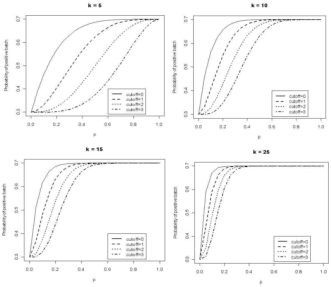 | Figure 3. Plot of  as a function of as a function of  for k = 5, 10, 15, 25 and l = 0, 1, 2, 3 when sensitivity and specificity = 70% for k = 5, 10, 15, 25 and l = 0, 1, 2, 3 when sensitivity and specificity = 70% |
The candidate  is dropped because it gives only two extreme solutions
  or
or  and thus
  or
or  . The estimate
  is most unlikely to happen since in practice it is not possible to avoid defectives and have only good items. On the other hand
  means that all the batches or items test positive which is certainly an overestimate of
  as it is most unusual for every item in the population to be positive (Hepworth and Watson, 2009). With the candidate
  we get;
 | (5) |
For l = 0, Equation (5) reduces to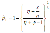 | (6) |
This is a result obtained by Nyongesa (2012). However, Equation (5) has no solution in closed form when  . Therefore, the equation is solved iteratively using an R code that we developed which is presented in Appendix A.
3. Properties of the Estimator
In this section, the properties of the maximum likelihood estimator of proportion are discussed.
3.1. Relationship between  and
and 
The relationship between  and
and  when the value of sensitivity and specificity of the test is fixed at 99% is presented in Figure 4. It can be noted that there is significant increase in the maximum likelihood estimate as the cut off value increases. But the increase diminishes with the increase in the batch size.
 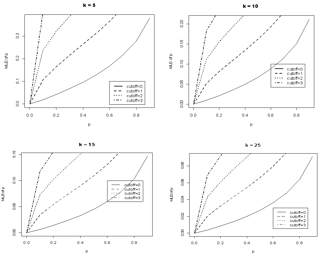 | Figure 4. Plot of  against against  for k = 5, 10, 15, 25 and l = 0, 1, 2, 3 with sensitivity and specificity = 99% for k = 5, 10, 15, 25 and l = 0, 1, 2, 3 with sensitivity and specificity = 99% |
The relationship is studied when the value of sensitivity and specificity is set at 95%. The results are shown in Figure 5 below.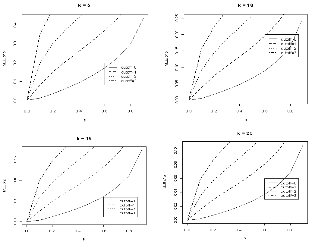 | Figure 5. Plot of  against against  for k = 5, 10, 15, 25 and l = 0, 1, 2, 3 with sensitivity and specificity = 95% for k = 5, 10, 15, 25 and l = 0, 1, 2, 3 with sensitivity and specificity = 95% |
The relationship is observed to be monotonically increasing and the rate of increment depends on k and l. Comparing Figures 4 and 5 it is found that the relationship is slightly affected by the values of sensitivity and specificity. Also to note is the fact that the Brookmeyer (1999) model gives lower estimates than the proposed model. This is indicated by the solid line lying below other lines.
3.2. Asymptotic Variance of Estimator
In this section, we consider the computation of the asymptotic variance of our estimator. The asymptotic variance is obtained from the Fisher’s information given by; | (7) |
And we obtain; | (8) |
where 
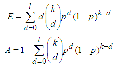 The derivation of Equation (8) is presented in Appendix B.The figures that follow below indicate the relationship between
  and
and  . The point of interest in the figures is to locate the region where the curves of the model with l > 0 are below the curve with l = 0 (solid line). That is, identify the region where the model is more efficient than the Brookmeyer (1999) model.As indicated in Figure 6, the Brookmeyer (1999) model is more efficient than the proposed model for small p. But the p for which the proposed model is more efficient than the Brookmeyer (1999) model reduces as k increases. For example, with k = 5, the proposed model is more efficient than Brookmeyer (1999) model for p > 0.3 while if k = 25, that value is p > 0.06. In Figure 7 the sensitivity and specificity was set at 95% and the relationship of
  with respect to p observed. The plot indicates that the p for which the proposed model is more efficient than the Brookmeyer (1999) model is relatively higher for small batch size as opposed to large batch size.
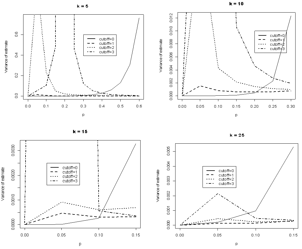 | Figure 6. Plot of  as a function of p for k = 5, 10, 15, 25 and l = 0, 1, 2, 3 with sensitivity and specificity = 99% as a function of p for k = 5, 10, 15, 25 and l = 0, 1, 2, 3 with sensitivity and specificity = 99% |
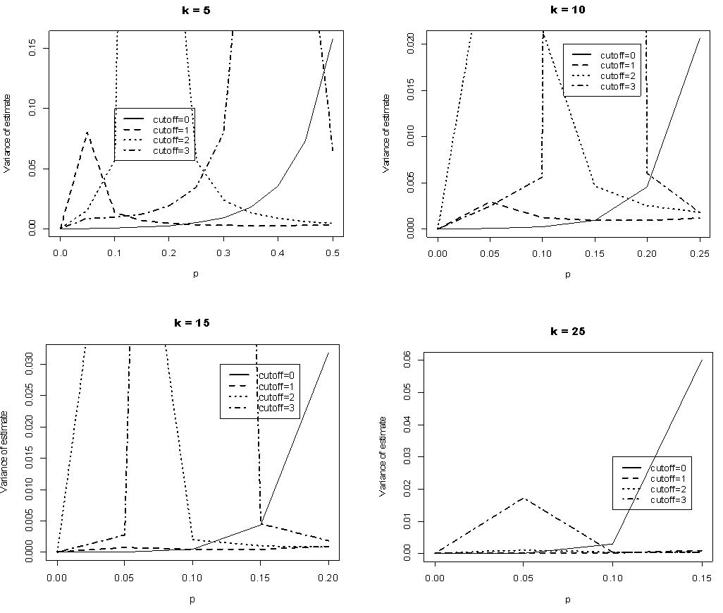 | Figure 7. Plot of  as a function of p for k = 5, 10, 15, 25 and l = 0, 1, 2, 3 with sensitivity and specificity = 95% as a function of p for k = 5, 10, 15, 25 and l = 0, 1, 2, 3 with sensitivity and specificity = 95% |
Comparing Figures 6 and 7 indicate that the proposed model is more efficient than Brookmeyer (1999) at lower p when sensitivity and specificity is low given small batches. For instance, if k = 5 and sensitivity and specificity = 99%, the proposed model is more efficient than Brookmeyer (1999) when p > 0.25. But when sensitivity and specificity = 95%, the model is more efficient with p > 0.21. However, if k is large, then p for which the proposed model is more efficient than the Brookmeyer (1999) model is relatively lower than one when both sensitivity and specificity are equal to 99% as opposed to when sensitivity and specificity are equal to 95%. For example, when k = 25 the proposed model is efficient compared to Brookmeyer (1999) when p > 0.01 if sensitivity and specificity is 99%. However, for the same batch size, the model is more efficient than Brookmeyer (1999) for p > 0.05 given the test has sensitivity and specificity equal to 95%.
3.3. Asymptotic Relative Efficiency
We compare our results with those of Brookmeyer (1999) among others by computing Asymptotic Relative Efficiency (ARE). If the estimator of Brookmeyer (1999) among others is denoted by  and our estimator
  by then
  | (9) |
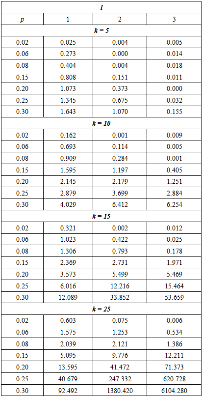
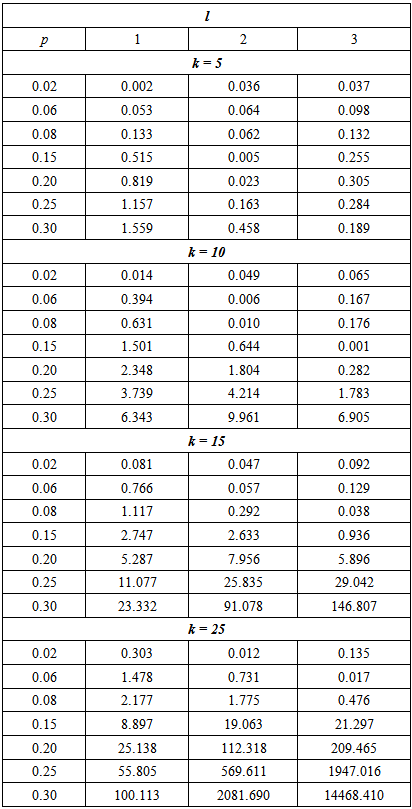
Therefore, ARE > 1 implies that the proposed model is more efficient than the Brookmeyer (1999) model. The tables that follow show ARE for some values of p with sensitivity and specificity equal to 99% and 95%.From Table 1, it can be seen that the proposed model is more efficient than Brookmeyer (1999) model for large values of p. However, the value of p for which our model is more efficient reduces with increase in k. Next sensitivity and specificity is reduced to 95% and the results are shown in the table below;Table 1. ARE of proposed model relative to Brookmeyer (1999) model for k = 5, 10, 15, 25 with sensitivity and specificity = 99%
 |
| |
|
The results in Table 2 indicate that the proposed model is more efficient than Brookmeyer (1999) model for relatively higher values of p as indicated by ARE > 1. Table 2. ARE of proposed model relative to Brookmeyer (1999) model for k = 5, 10, 15, 25 with sensitivity and specificity = 95%
 |
| |
|
3.4. Relative Mean Squared Error
If the estimator of Brookmeyer (1999) among others is denoted by  and our estimator
  by then the Relative Mean Squared Error (RMSE) is given by;
 | (9) |
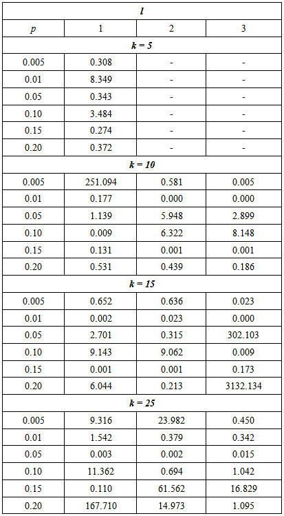
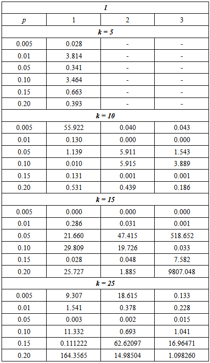
Table 3 gives the RMSE for a range of proportion values when the sensitivity and specificity is fixed at 99%.Table 3. MSE of the estimate for the proposed model relative to the Brookmeyer (1999) model with sensitivity and specificity = 99%
 |
| |
|
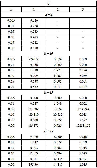
It can be seen that the efficiency of the proposed model depends on the p, k and l. For example, if p = 0.005 and l = 1, the proposed model is more efficient than Brookmeyer (1999) model when k = 10 or 25. But it is less efficient when k = 5 or 15.Next, the sensitivity and specificity is reduced to 95% and the RMSE calculated for a range of proportion and cut off values. The results are presented in Table 4.Table 4. The MSE of the estimate for the proposed model relative to the Brookmeyer (1999) model with sensitivity and specificity = 95%
 |
| |
|
The results indicate that the efficiency of the proposed model is reliant on the p, k and l. The proposed model performs better than the Brookmeyer (1999) model in several settings of p, l and k. But overall, the proposed model is more efficient when batch size increases.Lastly, the sensitivity and specificity was set to 90% and the models compared using the RMSE.From Tables 3, 4 and 5, it can be noted that the efficiency of the proposed model relative to the Brookmeyer (1999) model is affected by the value of sensitivity and specificity. However, the relationship between the relative efficiency of the proposed model and sensitivity and specificity is not a simple one. For instance, for large k = 15 and 25 with l = 1 and p = 0.05, the relative efficiency of the model is 2.701 increasing to 21.699 and then reducing to 21.660 for sensitivity and specificity equal to 99%, 95% and 90% respectively. Table 5. The MSE of the estimate for the proposed model relative to the Brookmeyer (1999) model with sensitivity and specificity = 90%
 |
| |
|
On the other hand if k = 10, the relative efficiency of the proposed model increases as the sensitivity and specificity increases. Therefore, one would need such tables to be able to set up a more efficient model provided that there is information about the proportion p, cut off value, l and sensitivity and specificity of tests.Note that RMSE could not be determined for k = 5 with l = 2 and 3 as indicated by missing values in Tables 3, 4 and 5. Hence for small batch size, k = 5, we should avoid large cut off values, l > 1.
4. Discussion and Conclusions
We have constructed an estimator for batch testing based on the quality control procedure in the presence of test errors. The probability of detecting a positive batch is much affected by the cut off value and batch size but least affected by sensitivity and specificity. The plots show significant increase in the probability of detecting a positive batch with increase in batch size for the given value of sensitivity and specificity. But the rate of increase diminishes with increase in the cut off value. The MLE of p derived is a generalization of one obtained by Nyongesa (2012) and has no closed form solution when l > 0. However, a computer code using an in-built R function, uniroot, is developed to determine the estimate of p. It is found out that the MLE of p increases with increase in sensitivity and specificity. It is also noted that the proposed model gives higher values for MLE of p than Brookmeyer (1999) model for fixed batch size, cut off value and sensitivity and specificity. If the sensitivity and specificity is assumed to be constant in the entire testing time, the proposed model improves the efficiency of the estimator over other models previously developed especially for higher values of p. The problem of errors in inspection can be mitigated by re-testing. It has been shown that re-testing of batches reduces misclassification errors (cf. Nyongesa, 2004). In fact, lost sensitivity of a test is recovered by re-testing batches classified as negative in the initial stage if the tests are imperfect. A batch testing model as applied in quality control where re-testing is allowed can be developed and investigated.
Appendix A: R Code to Determine MLE
#Program to find the estimate of p when test is imperfect#Specify the parameterk = 15x = 2l = 1n = 20d = c (0: l)Sensitivity = 0.99Specificity = 0.99#Define the function whose single root is to be determine in interval (0, 1)fun<-function(p) (sensitivity+specificity-1)*(sum(choose(k,d)*p^d*(1-p)^(k-d)))+x/n-sensitivityp.estimate<-uniroot(fun,c(0,1))$rootp.estimate
Appendix B: Derivation of Asymptotic Variance
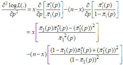
We consider the computation of the asymptotic variance of our estimator as presented in Equation (9). The variance is computed by solving for 
 But
But  | (10) |

 | (11) |
 Thus
Thus  | (12) |
Hence  | (13) |
where 
 and
and

References
| [1] | Biggerstaff, B. (2008). Confidence Intervals for the Difference of two proportions Estimated from Pooled samples. Journal of Agricultural, Biological and Environmental Statistics, 13, 478-496. |
| [2] | Brookmeyer, R. (1999). Analysis of Multistage Pooling Studies of Biological Specimens for Estimating Disease Incidence and Prevalence. Biometrics, 55, 608-612. |
| [3] | Chen, H. and Bonis, A. D. (2011). An almost Optimal Algorithm for Generalized Threshold Group Testing with Inhibitors. Journal of Computational Biology, 18, 851-864. |
| [4] | Damaschke, P. (2006). Threshold Group Testing. Information Transfer and Combinatorics, Lecture notes in Computer Science, 4123, 707-718. |
| [5] | Dorfman, R. (1943). The detection of defective members of large population. Annals of Matematical Statistics, 14,436-440. |
| [6] | Hepworth, G. (1999). Estimation of Proportions by Group Testing. PhD thesis, University of Melbourne. |
| [7] | Hepworth, G. and Watson, R. (2009). Debiased Estimation of Proportions in Group Testing. Applied Statistics, 58, 105-121. |
| [8] | Hughes-Oliver, M. J. (2006). Pooling Experiments for Blood Screening and Drug Discovery. Screening: Methods for Experimentation in Industry, Drug Discovery and Genetics, New York, Springer. |
| [9] | Hughes-Oliver, M. J. and Swallow, H. W. (1994). A Two-Stage Adaptive Procedure for Estimating Small Proportions. Journal of the American Statistical Association, 89, 982-993. |
| [10] | Montegomery, D. C. (2009). Introduction to Statistical Quality Control (6th edition). New York, John Wiley and Sons. |
| [11] | Nyongesa, L. K., (2004). Multistage Group testing procedure (Batch screening). Communication in Statistics-Simulation and Computation, 33, 621-637. |
| [12] | Nyongesa, L. K., (2012). Dual Estimation of Prevalence and Disease Incidence in Pool-Testing Strategy. Communication in Statistics Theory and Method. 40, 1-12. |
| [13] | Sobel, M., and Elashoff, R.M., (1975). Group -testing with a new goal, Estimation. Biometrika, 62, 181-193. |
| [14] | Thomson, K. H. (1962). Estimation of the Proportion of Vectors in a Natural Population of Insects, Biometrics, 18, 568-578. |
| [15] | Tu, M. X., Litvak, E. and Pagano, M. (1995). On the Informative and Accuracy of Pooled Testing in Estimating Prevalence of a Rare Disease: Application to HIV Screening. Biometrika, 82, 287-297. |


 and
and  are sensitivity and specificity of the test, then the probability of classifying a batch as positive;

 and
and  by plotting
  against
  for different k and l. The value of sensitivity and specificity is fixed and assumed equal in the course of testing. Figure 1 shows the relationship between
  versus
  given that the sensitivity and specificity are equal to 99%. It can be noted that the probability increases rapidly for low p converging to the value of sensitivity.
 as a function of
  for k = 5, 10, 15, 25 and l = 0, 1, 2, 3 with sensitivity and specificity = 99%
 as a function of
  for k = 5, 10, 15, 25 and l = 0, 1, 2, 3 with sensitivity and specificity = 90%
 and p is least affected by the values of sensitivity and specificity.
  . Thus the likelihood function is;

 In solving Equation (4), there are two possible solutions;

 as a function of
  for k = 5, 10, 15, 25 and l = 0, 1, 2, 3 when sensitivity and specificity = 70%
 is dropped because it gives only two extreme solutions
  or
or  and thus
  or
or  . The estimate
  is most unlikely to happen since in practice it is not possible to avoid defectives and have only good items. On the other hand
  means that all the batches or items test positive which is certainly an overestimate of
  as it is most unusual for every item in the population to be positive (Hepworth and Watson, 2009). With the candidate
  we get;

 . Therefore, the equation is solved iteratively using an R code that we developed which is presented in Appendix A.
 and
and 
 and
and  when the value of sensitivity and specificity of the test is fixed at 99% is presented in Figure 4. It can be noted that there is significant increase in the maximum likelihood estimate as the cut off value increases. But the increase diminishes with the increase in the batch size.
 against
  for k = 5, 10, 15, 25 and l = 0, 1, 2, 3 with sensitivity and specificity = 99%
 against
  for k = 5, 10, 15, 25 and l = 0, 1, 2, 3 with sensitivity and specificity = 95%


 The derivation of Equation (8) is presented in Appendix B.The figures that follow below indicate the relationship between
  and
and  . The point of interest in the figures is to locate the region where the curves of the model with l > 0 are below the curve with l = 0 (solid line). That is, identify the region where the model is more efficient than the Brookmeyer (1999) model.As indicated in Figure 6, the Brookmeyer (1999) model is more efficient than the proposed model for small p. But the p for which the proposed model is more efficient than the Brookmeyer (1999) model reduces as k increases. For example, with k = 5, the proposed model is more efficient than Brookmeyer (1999) model for p > 0.3 while if k = 25, that value is p > 0.06. In Figure 7 the sensitivity and specificity was set at 95% and the relationship of
  with respect to p observed. The plot indicates that the p for which the proposed model is more efficient than the Brookmeyer (1999) model is relatively higher for small batch size as opposed to large batch size.
 as a function of p for k = 5, 10, 15, 25 and l = 0, 1, 2, 3 with sensitivity and specificity = 99%
 as a function of p for k = 5, 10, 15, 25 and l = 0, 1, 2, 3 with sensitivity and specificity = 95%
 and our estimator
  by then
 and our estimator
  by then the Relative Mean Squared Error (RMSE) is given by;

 But
But 


 Thus
Thus 


 and
and

 Abstract
 Reference
 Full-Text PDF
 Full-text HTML