1. Introduction

Studies on climatic conditions have increased significantly in the past decades as a result of advances in observational, analysis, and modelling capabilities. Moreover, [1] report on climate change has rekindled research interest. Various applicable techniques are being employed by researchers to help in understanding the phenomenon of climate change. [2] remarked that the use of the state-of-the-art statistical methods could substantially improve the quantification of uncertainty in assessments of climate change. [3] concluded that empirical-statistical downscaling can be viewed as part of an analysis that provide valuable diagnostics that can illuminate various aspects of Global Climate Models (GCMs) and complements nested modelling and provides a valuable independent approach for studying local climate. [4] In a comparative study of statistical and neuro-fuzzy network models for forecasting the weather of Goztepe, Istanbul using Adaptive Neuro-Fuzzy Inference System (ANFIS) and Autoregressive Integrated Moving Average (ARIMA) models, ANFIS performed slightly better than ARIMA evaluating the RMSE and R². [5] created a statistical model that is based on variables known to be important for deterministic models that can be used to forecast water temperature as a response to atmospheric conditions and reported a daily average model with R² > 0.93 during verification periods. [6] used non-stationary multivariate geo-statistical techniques for the prediction of annual mean air temperature and precipitation data using kriging-based prediction. In comparison with linear regression-based prediction, the kriging-based performed better, yielding mean square error lower by 53-75%.

Literature study for Africa and Europe on climate parameters is skewed towards the analysis of rainfall ([7]; [8]; [9]; [10]; [11]). In Ghana, climate studies have been conducted and reported in literature. [12] in studying the effect of declining rainfall in the White and Oti Volta Basins on the Akosombo Dam, partially considered the mean monthly variation in air temperature and reported, prior to 1% rise from 1945 to 1993, that there has been increase in evaporation as a result of this rise in temperature. Quantification of the increase was however not specified. [13] reported that Ghana’s average surface temperature as 26°C but indicated that there had not been any significant change in trend over the period of 1963 to 1992. However, [14] reported a global increase by about 0.7°C and [1] reported pre-industrial temperatures rise by 0.8°C with ocean temperatures rising by 0.09°C, an evidence of global warming. [16] predicted a rising mean annual temperature change of 0.8°C in Ghana. A likely temperature rise of 4°C has been predicted by [1]. In a related study, [16] concluded on SARIMA (2,1,1)×(1,1,2)₁₂ as the best model for forecasting the monthly mean surface temperature of the Ashanti Region of Ghana. This study focused on building a statistical model for forecasting the monthly average surface temperature in the BA region of Ghana to help in understanding the dynamics of events. The paper is organised into four sections, the first section introduces the subject by reviewing some relevant literature; the second section discusses the methods and materials used for the data analysis, the Box-Jenkins Algorithm, stationarity and nom-stationarity of time series data, model types are presented under section two; findings and discussions of results will be presented under section three; and the fourth section will conclude the paper by highlighting major findings.

2. Method and Materials

2.1. Box Jenkins Algorithm

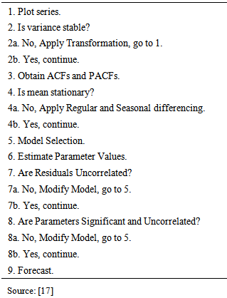
The approach is to use data in the past to provide forecasts. Using the ARIMA self-projecting time series forecasting model, we hope to find a mathematical formula that will approximately generate the historical patterns in a time series. The self-projecting time series uses only the time series data of the activity to be used to generate forecasts. This approach is typically useful for short to medium-term forecasting [17]. The underlying goal of the Box-Jenkins Forecasting Method is to find an appropriate formula so that the residuals are as small as possible and exhibit no pattern. The model-building process involves four steps, repeated as necessary, to end up with a specific formula that replicates the patterns in the series as closely as possible and also produces accurate forecasts. This process is outlined in Table 1.

Table 1. Box-Jenkins Modelling Algorithm

2.2. Stationarity and Non-Stationarity of Time Series Data

The stationarity of the n-th order time series is established if

(1.1)

for all and all This implies that the joint distribution is invariant to time shift by k for all n= 1,2,.... (1.1) depicts a time series as strictly stationary. The converse is true for non-stationary. If (1.1) is true for it is also true for because the m-th order distribution function determines all distribution functions of lower, hence a high order of stationarity always implies a lower order of stationarity [18]. Mostly, a weaker sense of stationarity is defined in theory and practice. A process is said to be n-th order weakly stationary if all its joint moments up to order n exist and are time invariant.

Stationarity plays a crucial role in time series analysis. One can test the stationarity or otherwise of a time series data using the unit root test proposed by Dickey and Fuller in 1979, for testing the hypothesis below;

If the ADF test statistic is less than the critical value, we fail to accept H₀. The test is based on the fact that for stationarity to exist, the roots of the characteristics polynomial of the time series must lie outside a unit circle.

2.3. Model Types

2.3.1. Autoregressive Models of order p [AR(p)]

The p-th order autoregressive process is given by;

(2)

with auto-covariance function,

(3)

and a recursive relation for the autocorrelation function,

(4)

The process is stationary if the roots of lie outside a unit circle. The pacf vanishes after lag p.

2.3.2. Moving Average Process of Order q [MA(q)]

The q-th order moving average process is

(5)

The MA(q) process is always stationary because The process is invertible if the roots of lie outside a unit circle.

The auto-covariance function is given by

(6)

Therefore, the autocorrelation function becomes

(7)

The autocorrelation function of an MA(q) process cuts off after lag q.

2.3.3. Autoregressive Moving Average (p,q) Process

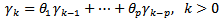
Let

A zero-mean ARMA(p,q) process is then defined as

(8)

The process is invertible and stationary if the roots of respectively lie outside the unit circle.

For we get an auto-covariance function of

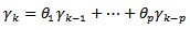(9)

and an autocorrelation function of

(10)

2.3.4. Autoregressive Integrated Moving Average (p,d,q) Process

A time seires is said to be homogeneous non-stationarity if is stationary for some value of A stationary ARMA(p,q) model for is given by

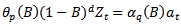(11)

Equation (11) is called autoregressive integrated moving average model, ARIMA(p,d,q).

2.3.5. Seasonal ARIMA (SARIMA) Models

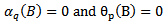
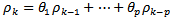
SARIMA models are an adaptation of autoregressive integrated moving average (ARIMA) models to specifically fit seasonal time series. That is, their construction takes into consideration the underlying seasonal nature of the series to be modelled. Many authors have written on SARIMA models extensively. A few amongst them are [18] who proposed them, [19], [20], [21] and [22].

SARIMA model is written as follows:

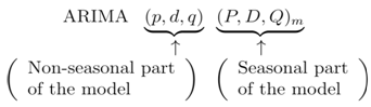where m = number of periods per season, the uppercase notation for the seasonal parameters of the model, and lowercase notation for the non-seasonal parameters of the model. The seasonal part of the model consists of terms that are very similar to the non-seasonal components of the model, but they involve backshifts of the seasonal period.

A multiplicative seasonal ARIMA model is given by;

(12)

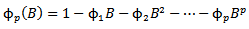
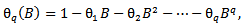
where and are defined as;

(13)

(14)

where

(15)

where

(16)

where s is an integer strictly larger than one (the period), and Note that For example, an ARIMA(1,1,1) × (1,1,1)₄ model (without a constant) is for quarterly data (m=4) and can be written as;

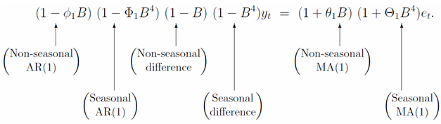The additional seasonal terms are simply multiplied with the non-seasonal terms.

3. Findings and Discussions

In this section, outputs from data exploration and employing the Box-Jenkins Algorithm in building a model are presented and discussed. The data employed in this study were collected from the Department of Meteorology and Climatology in the BA Region, and represent the monthly rainfall figures from January 1975 through December 2009. The data was used since it is a time series data and the observations were collected sequentially in time (monthly). Data was analysed with RStudios 0.98.1062. The 420 data points for the time period observed are presented in Figure 3.

3.1. Preliminary Data Analysis

An exploratory routine was employed to reveal some important features in the data set. Figure 1 presents the yearly mean surface temperature from 1975 to 2009. From Figure 1 no pattern to trend can be concluded on, however average surface temperature has experienced some rise and fall in figure over the years. The average surface temperature observed lies between 23°C and 32°C. The least yearly average surface temperature of 23.7°C within the period was observed in 1976, and the highest figure of 31.5°C was observed in 1999. There seems to be a downward trend from 2007.

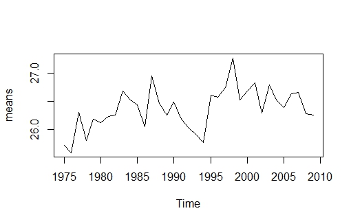Figure 1. Distribution of the yearly average surface temperature from 1975 to 2009

The average monthly surface temperature for the period was examined. Figure 2 presents the descriptive indicators worthy of examining in a boxplot.

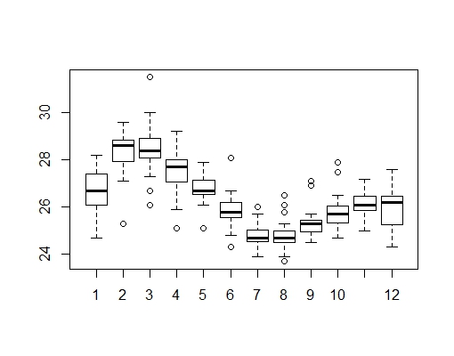Figure 2. Boxplot of the monthly average surface temperature from Jan. 1975 to Dec. 2009

The data considered on monthly basis has many outliers, with exception of the months of January, November and December. This requires some smoothening to be performed to remove the effort of the outliers. The month of February recorded the highest average surface temperature, followed closely by March, which had the highest upper quartile value as well as the largest outlier value. The high values could be associated to the severe dry weather experience during those times of the year. The months of July and August recorded the least average surface temperature values. This may be associated to the numerous downpour experienced during those times of the year. It can be observed from chart that the average figure start increasing from September through to February and then it starts dropping from March through to August.

The time series plot for the monthly average surface temperature for the Brong Ahafo from January 1975 to December, 2009 is presented in Figure 3. The data look stationary by observation from Figure 3. However, the regular pattern of up and down in Figure 1 is an indication of seasonality. Figure 3 was further investigated by decomposing it into the various components. The decomposed plots of the various components of the time series plot in Figure 1 is as presented in Figure 4.

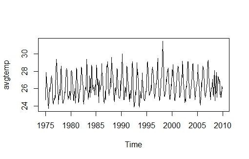Figure 3. Time Series plot for Monthly Average Temperature from Jan. 1975 to Dec. 2009

From Figure 4, the data has seasonal effect, with a usual rise and fall pattern being experienced yearly over the period. This implies that regular average surface temperature recorded each year was influenced by the rise and fall pattern of the seasonality component. However, the trend seems to be very constant over time, although there are a few ups and downs over some periods. The random effect is very stable over the time period, although one could be interest in its erratic nature between 2007 and 2009.

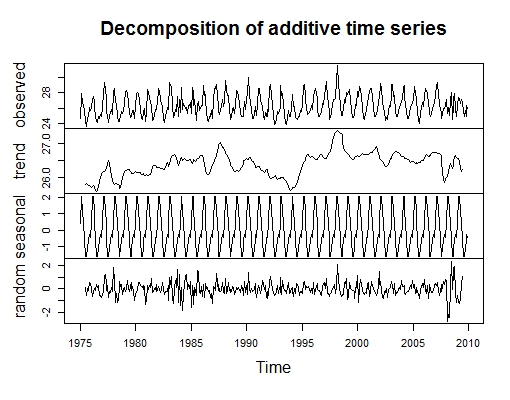Figure 4. Decomposed Time Series plot for Monthly Average Temperature from Jan. 1975 to Dec. 2009

3.2. Stationarity Test

A formal statistical test is performed at this stage to ascertain the stationarity or otherwise of the data. The hypotheses under consideration are;

H₀: The data is stationary vrs H₁: The data is explosive

The Augmented Dickey-Fuller test reported a test value of -3.493 and a p-value of 0.9567. This result presents evidence in favour of the null hypothesis, postulating that the data is stationary.

3.3. ARIMA Model Fit to the Data

The Box-Jenkins Algorithm is an iterative scheme which mainly involves model identification, model estimation, models’ goodness of fit and model forecasting.

3.3.1. Model Identification

A closely examination was conducted on the Autocorrelation Functions (ACF) and Partial Autocorrelation Functions (PACF) plots in Figure 5. The ACF plot depicts a sine wave with very slow tailing off property. The spikes at lags 1, 12 and 24 are highly significant supporting the earlier evidence of seasonality in the data. Therefore the need for seasonal differencing with period of 12 is required to remove the effect of seasonality. The time series, ACF and PACF plots for the seasonally differenced data are presented in Figure 6.

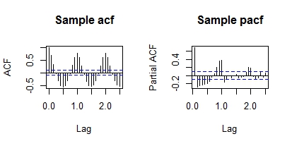Figure 5. ACF and PACF plots for Monthly Average Temperature from Jan. 1975 to Dec. 2009

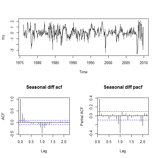Figure 6. Time Series, ACF and PACF plots for the Seasonally Differenced Monthly Average Temperature from January 1975 to December 2009

From Figure 6, the ACF at lags 1 and 2 are significant since the spikes passes out of the confidence limits. Hence the order of the non-seasonal MA term is 2. The seasonal MA terms occurs at lags which are multiples of 12. Only lag 12 spike is significant. Hence the order of seasonal MA term is 1. Similarly, a significant spike at lag 1 in the PACF indicates possible non-seasonal AR terms. The order of the non-seasonal AR part is 1 and 2 lags at multiples of 12 the seasonal part of the AR are significant, and that the seasonal AR is 2. Therefore the initial suggestion of an ARIMA (1, 0, 2) (2, 1, 1) ₍₁₂₎ is proposed. However, studies of neighbouring models to the proposed model suggest an ARIMA (1, 0, 0) (0, 1, 2) ₍₁₂₎ as the best alternative. 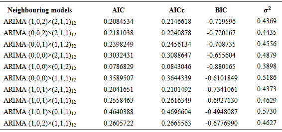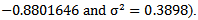Comparing the various selection criteria indicators, ARIMA (1,0,0) (0,1,2)₍₁₂₎ recorded the least value among all indicators considered Table 2 presents summary of the results.

Table 2. Summary of model identification

In fitting the model, the dataset was divided into training and test set. Observations from January 1975 to December, 2007 were used as the training set and were use to model a fit for the phenomenon under study. Data from January 2008 to December 2009 were designated as the test set and was used to assess the predictability accuracy of the fit. The result of the fit is as presented in Table 3.

Table 3. Parameter estimation of ARIMA (1,0,0)×(0,1,2)12

Model parameters are all significant at 5% level of significance, with an MSE of 0.3898, as can be found in Table 3.

3.4. Model Diagnostics

From theory, it is expected that autocorrelation functions of the residuals out of which less than 5% spikes should be noticed for the residuals to be accepted as a white noise. However, from Figure 7, almost all the spikes of the ACF and PACF plots all lie within the confidence bounds suggesting that the residuals are white noise. The normal q-q plot seems ok, because most of the dataset lie on the straight line. Much conviction of normality of the residuals of the fitted model is established by observing the histogram of the residuals of the fit presented in Figure 8. The bell-shape feature is clearly noticed in Figure 8, indicating that the residuals are normally distributed. A further analysis was conducted to ascertain the certainty of the residuals being white noise. A Box-Ljung test was reported a (df = 12) with a large p-value = 0.7219, suggesting that the residuals are white noise.

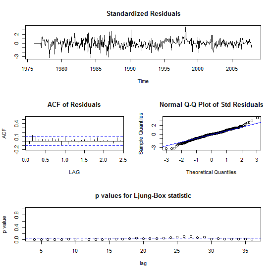Figure 7. Time Series, ACF and PACF plots for the Residuals of the Seasonally Differenced Monthly Average Temperature from January 1975 to December 2007

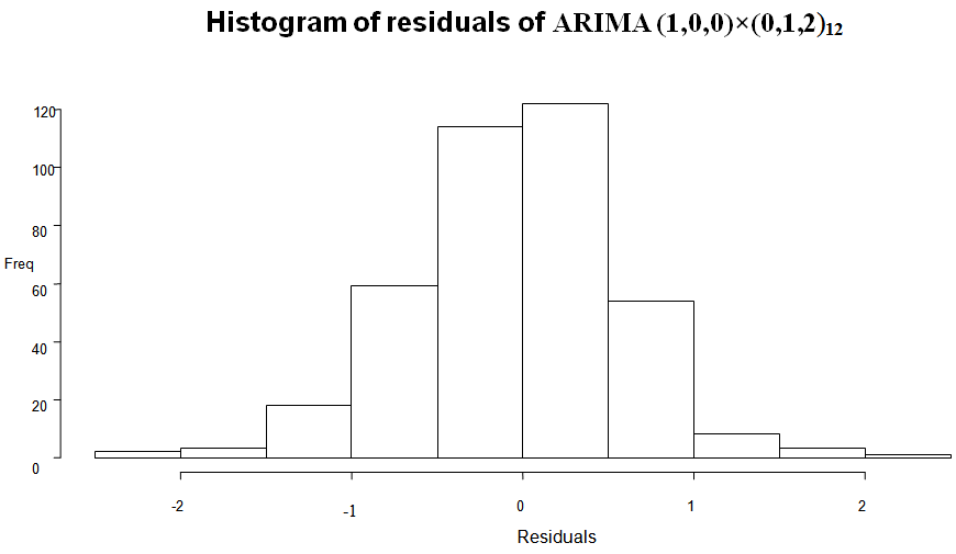Figure 8. Distribution of the residuals of ARIMA (1,0,0)×(0,1,2)12

3.5. Forecasting

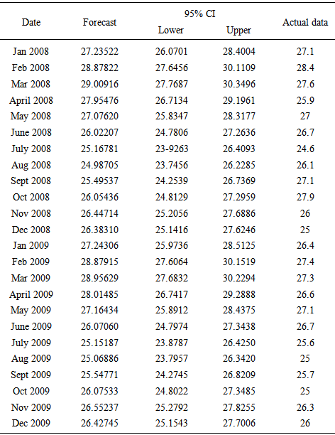
From Table 4, the predicted values are compared with the test data.

Table 4. A Twelve step forecast values with Standard Errors

From Table 4, the forecasted figures from SARIMA (1,0,0)×(0,1,2)₁₂ tends to be very close to the actual data, used as test data. The actual figures lied within the 95% confidence interval in most cases, over 85% of them lied within the forecasted interval. Visualization can be made by observing Figure 9. The model predicts well.

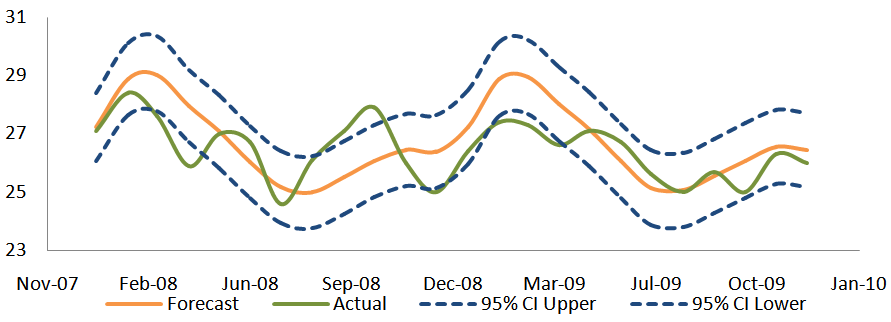Figure 9. The plot of the SARIMA (1,0,0)×(0,1,2)12 forecasted values and the actual figures observed

4. Conclusions

The average surface temperature observed lies between 23°C and 32°C for the Brong Ahafo region all year. The month of February records the highest average surface temperature in the region, with July and August sharing spot as the months that usually record the lowest average surface temperature. The mean yearly surface temperature over the period was quite erratic however a decreasing trend was from 2007 to 2009. SARIMA (1,0,0)×(0,1,2)₁₂ has been identified as an appropriate model for predicting monthly average temperature for the Brong Ahafo Region of Ghana. A monthly average surface temperature of 30°C is experienced by the Brong Ahafo Region of Ghana and the technocrats can estimate the amount of solar irradiance that can be generated and the amount of kilowatts of energy feasible. It is the hope that when the findings are adopted by the Ghana Metrological Agency and other relevant organisations, it will in the long run help in accurate forecasting and education of the populace on surface temperature.