Nasiru M. O., Olanrewaju S. O.
Department of Statistics, University of Abuja, Abuja, Nigeria
Correspondence to: Nasiru M. O., Department of Statistics, University of Abuja, Abuja, Nigeria.
| Email: |  |
Copyright © 2015 Scientific & Academic Publishing. All Rights Reserved.
Abstract
This research fit a univariate time series model to the Airline Fatalities in the world from 1920 through 2013. The Box-Jenkins Autoregressive Integrated Moving Average (ARIMA) Model was estimated and the best fitting ARIMA model was used to obtain the post-sample forecasts for five years. The fitted model for the Fatalities was ARIMA (0,1,1) with BIC of 12.375, Stationary R2 of 0.416, and MLE of 243.390. This model was further validated by Ljung-Box test with no significant Autocorrelation between the residuals at different lag times and subsequently by white noise of residuals from the diagnostic checks performed which clearly portray randomness of the standard error of the residuals, no significant spike in the residual plots of ACF and PACF. The forecasts value indicates that Airline Fatalities will increase insignificantly for the next five years (2014-2018).
Keywords:
ARIMA, Time Series, Box- Jenkins, Ljung-Box, Stationarity, Unit Root, Airline Fatalities, Forecast
Cite this paper: Nasiru M. O., Olanrewaju S. O., Forecasting Airline Fatalities in the World Using a Univariate Time Series Model, International Journal of Statistics and Applications, Vol. 5 No. 5, 2015, pp. 223-230. doi: 10.5923/j.statistics.20150505.06.
1. Introduction
Airline accidents are paramount issue in the contemporary airline industry, since they have a significant impact on the demand for air travel, affecting the finances of the airlines. If travelers believe that an air travel incident is a random event, then they will pay little attention to it, since it does not reveal any further information on air travel safety. However, if they believe that it is not a random event, then air travel is perceived as dangerous and passengers switch for a safer airline or choose an alternative traveling mode. This issue has been examined among others by Rose, Nancy L. (1992), Borenstein and Zimmerman (1988), Bosch et al. (1998).Literature has shown that previous research on Airline accidents focused on the effect of fatal accident on the equity values of Airlines. For example, Borenstein and Zimmerman (1998), Mitchell and Maloney (1989), Bosch et al (1998). They also examined the impact of fatal accidents on Air travel demand. Their results showed that fatal accident have a significant negative effect on the stock value of the Airlines involved in such accidents. Other results showed that fatal accidents have no significant effect on the equity values of other Airlines. Mitchell and Maloney (1989), in their research, found out that equity value of the Airline involved in a fatal accidents falls only if the accidents is the fault of the company. Their findings further showed that; if the financial market is perfect, the stock value of the Airline should have already considered the expected responses of the demand. Their s findings may suggest that fatal accidents have little impact on the total demand for Air travel. Borenstein and Zimmerman (1988), further examined the impact of fatal accidents on the demand for Air of crash Airlines remained largely unaffected by the fatal accidents prior to deregulation.Airline fatalities data can be viewed as a count data which has been primarily categorized as cross-sectional time series, and panel count data. Over the past decades, Poisson and Negative Binomial (NB) models have been used widely to analyse cross-sectional and time series count data, and random effect and fixed effect Poisson and NB models have been used to analyse panel count data. However, in recent time, literature suggests that although the underlying distributional assumptions of these models are appropriate for cross-sectional count data, they are not capable of taking into account the effect of serial correlation often found in pure time series count data. Real-valued time series models, such as the autoregressive integrated moving average (ARIMA) model, introduced by Box and Jenkins have been used in many applications over the last few decades. However, when modeling non-negative integer-valued data where the dataset is relatively low (less than 30 Observations) such as traffic accidents over time, Box and Jenkins models may be inappropriate. This is mainly due to the normality assumptions of error in the ARIMA model. Over the last few years, a new class of time series models known as integer-valued autoregressive (INAR) Poisson models has been studied by many authors. This case of model is particularly applicable to the analysis of time series count data as these models hold the properties of Poisson regression and able to deal with serial correlation, and therefore offers an alternative to the real-valued time series models.Mohammed A. Quddus (2008), introduced the class of INAR models for the time series analysis of traffic accidents in Great Britain. He compared the performance of the INAR models with the class of Box and Jenkins real-valued models, his result suggest that the performance of these two classes of models is quite similar in terms of coefficients estimates and goodness of fit for the case of aggregated time series traffic accidents data. This is because the mean of the counts is high in which case the normal approximations and the ARIMA models may be satisfactory.Mohammed A. Quddus (2008), in his work, developed accident prediction models of a highly aggregated time series process of annual road traffic fatalities in Great Britain. He employed a range of econometrics models such as ARIMA, NB, and INAR Poisson models. He investigated the performance of the fitted models. His result implied that the best accident prediction model for the aggregated time series count data was achieved when ARIMA model was used. This is due to the fact that this model is able to take into account both serial correlation and non-stationarity normally found in a time series dataset. The objectives of this research are: (i) to evaluate the pattern and duration of the airline fatalities in the world from 1920 through 2013 (ii) to fit a univariate time series ARIMA model for Airline fatalities and (iii) use the fitted model to make five years forecast.George E.P. Box and Gwilym M. Jenkins (1970) integrated the existing knowledge on time series with their book “Time Series Analysis: Forecasting and Control”. First of all, they introduced univariate models for time series which simply made systematic use of the information included in the observed values of time series. This offered an easy way to predict the future development of the variable. Moreover, these authors developed a coherent, versatile three-stage iterative cycle for time series identification, estimation, and verification.George E.P. Box and Gwilym M. Jenkins (1970) book had an enormous impact on the theory and practice of modern time series analysis and forecasting. With the advent of the computer, it popularized the use of autoregressive integrated moving average (ARIMA) models and their extensions in many areas of science. Since then, the development of new statistical procedures and larger, more powerful computers as well as the availability of larger data sets has advanced the application of time series methods, the autoregressive and moving average models have been greatly favored in time series analysis. Simple expectations models or a momentum effect in a random variable can lead to AR models. Similarly, a variable in equilibrium but buffeted by a sequence of unpredictable events with a delayed or discounted effect will give MA mode.
2. Methodology and Model Specification
The model used in this study is the ARIMA proposed by Box and Jenkins (1976). The preliminary test for stationarity and seasonality of the data was conducted in which differences (d) as well as transformation were taken. After the stationarity of the series was attained, ACF and PACF of the stationary series are employed to select the order p and q of the ARIMA model. At this stage, different candidates’ model manifested and their parameters were estimated using the maximum likelihood method. Based on the model diagnostic tests and parsimony we obtained the best fitting ARIMA model. The Mathematical model for Auto Regressive of order p as well as that of Moving Average of order q are given respectively as  | (1) |
and | (2) |
The ARMA process of order (p,q) is written as  | (3) |
Method of Estimation: ARIMA MethodologyThe Box-Jenkins model building techniques consists of the following four steps:Step 1: Preliminary Transformation: If the data display characteristics violating the stationarity assumption, then it may be necessary to make a transformation so as to produce a series compatible with the assumption of stationarity. After appropriate transformation, if the sample autocorrelation function appears to be nonstationary, differencing may be carried out.Step 2: Identification: If yt is the stationary series obtained in step 1, the problem at the identification stage is to find the most satisfactory ARMA (p,q) model to represent yt Box – Jenkins (1976) determined the integer parameters (p,q) that govern the underlying process yt by examining the autocorrelations function (ACF) and partial autocorrelations (PACF) of the stationary series, yt. This step is not without some difficulties and involves a lot of subjectivity. It does on occasion happen that evidence examined at this stage may not point clearly in the direction of a single model (Salau, 1998). Hence, it is useful to entertain more than one structure for further analysis. Salau (1998) stated that this decision can be justified on the ground that the objective of the identification phase is not to rigidly select a single correct model but to narrow down the choice of possible models that will then be subjected to further examination.Step 3: Estimation of the model: This deals with estimation of the tentative ARIMA model identified in step 2. The estimation of the model parameters can be done by the conditional least squares and maximum likelihood.Step 4: Diagnostic checking: Having chosen a particular ARIMA model, and having estimated its parameters, the adequacy of the model is checked by analyzing the residuals. If the residuals are white noise; we accept the model, else we go to step 1 again and start over.
3. Analysis and Results
TIME SERIES GRAPH OF THE RAW DATA Time series plots which display observations on the y-axis against equally spaced time intervals on the x-axis used to evaluate patterns and behaviors in data over time for Airlines fatalities in the world is displayed in the Figure 1 below. The data used for this research was sourced from www.airdisasters.co.uk from 1920 through 2013.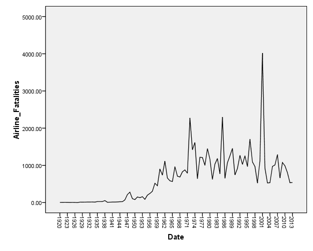 | Figure 1. Time Series Graph of Airline Fatalities 1920 - 2013 |
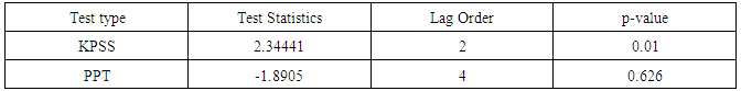
Table 1. Unit Root and Stationarity Tests of Airline Fatalities
 |
| |
|
4. Discussion of Result
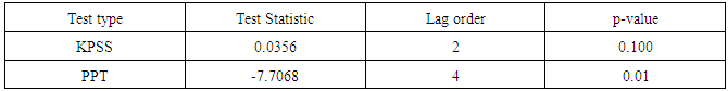
The time series plots of the raw data as displayed in Figure 1 indicates clearly that the occurrence of major Airline Fatalities in the world from 1920 through 2013 was not constant but rather varied from one year to the other with no systematically visible pattern, structural breaks, outliers, and no identifiable trend components in the time series data or non monotonous (that is consistently increasing or decreasing), this behaviors clearly revealed that non- stationarity was inherent in the data. The unit root tests provide a more formal approach to determining whether the series is stationary or not such as Kwiatkowski-Phillips-Schmidt-Shin (KPSS) and Phillips-Perron Unit Root Tests (PPT), these were carried out as shown in Table 1, we employed the unit root testing procedures of Hamilton (1994). The KPSS test statistic of a p -values which is less than the critical value of 0.05 as presented in Table 1 rejects the null hypothesis of having a level stationary series and therefore conclude the alternate hypothesis that it has a unit root. Philips-Peron Test on the other hand, fails to reject the null hypothesis at 5% significance level, since its p-values were greater than 0.05. It is clear from the time series plot of Airline Fatalities and the unit root test that the series has to be transformed or differenced to stabilize or stationarize the data before its capability is assessed or improvements are initiated. The time series of the first difference in Figure 2 does appear to be stationary in mean and variance, as the level of the series stays roughly constant over time. It is clear that the mean is exactly zero which confers a stationary series. The unit root test which is a formal method of testing the stationarity of a series was subsequently performed to augment the graphical analysis already performed since ignoring the problem of the unit root will cause an error with the statistical inference. Table 2 depicts the KPSS and the PPT for the first order differenced of the series, The KPSS test statistic of a p-values which are greater than the critical value of 0.05 do not reject the null hypothesis of having a level stationary series. Philips-Peron Test on the other hand test statistic and its p-values reject the null hypothesis of a unit root at 5% significance level, since its p-values are less than 0.05. It therefore can be concluded that the time series plot of the first differenced indicates that the series was stationary at first difference. | Figure 2. FIRST Order Difference of Airline Fatalities |
Table 2. Unit Root and Stationarity Tests for the Differenced of Airline Fatalities
 |
| |
|
Figures 3 comprised the plot of ACF and PACF. If the PACF displays a sharp cutoff while the ACF decays more slowly (i.e., has significant spikes at higher lags), we say that the series displays an AR signature, however, if the ACF displays a sharp cutoff while the PACF decay more slowly, we say that the series displays an MA signature. The lag at which the ACF cuts off is the indicated number of MA terms. It can be seen from Fig 3 that there is a slow decay in the PACF, but has a cut-off at lag1, lag2, lag3 and lag4 suggesting AR(1), AR(2) AR(3) and AR(4) respectively, the ACF has two significant spike at lag 1 and lag 16, This pattern is typical to a Moving Average (MA) process of order 1 and 16, but the parameter of that of order 16 was not significant, and was not included in the model. Hence a number of possible models identify themselves, these models are: ARIMA (1,1,1), ARIMA (2,1,1), ARIMA (3,1,1), ARIMA (4,1,1), and ARIMA(0,1,1). We proceeded to further statistically analyzed these five possible models and the results were summarized in the table 3.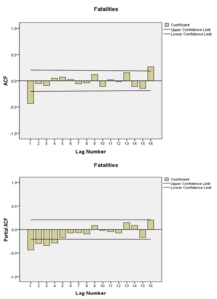 | Figure 3. Plots of ACF and PACF of Major Airline Disasters |
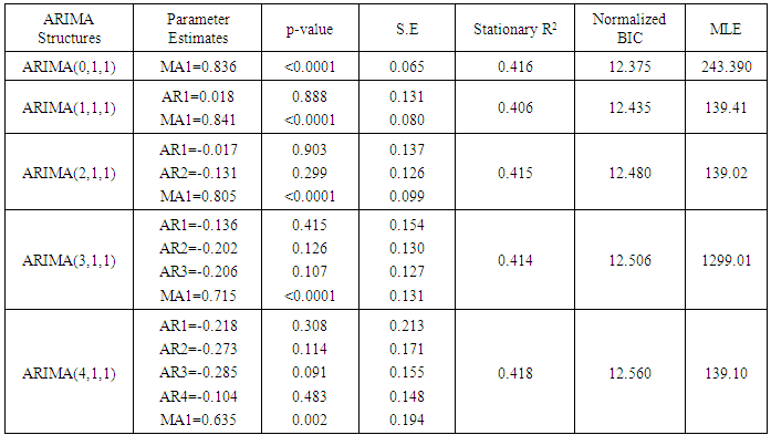
Table 3. ARIMA Models Results
 |
| |
|
Based on the parameters estimates as reported in Table 3 of major Airline Fatalities, the estimate of all the AR models were found to be statistically insignificant because their p-value were all greater than 0.05 Therefore the null hypothesis (Ho) of parameter are or equal zero is not rejected resulting in their removal from the model. The estimates of the MA model on the other hand, was found to be statistically significant because it p-value is less than 0.05 significance level. Additionally, comparing the ARIMA (0,1,1), ARIMA (1,1,1), ARIMA (2,1,1), ARIMA (3,1,1), ARIMA (4,1,1), models in terms of the Stationary R2, BIC, MLE respectively, clearly prefer ARIMA (0,1,1) model since It has highest Stationary R2, smallest BIC, and highest MLE. The summary of the estimates of ARIMA (0,1,1) is given in table 3. Based on the parameter estimates in the Table 3 chose the ARIMA (0,1,1) as the best model for the Airline Fatalities in the world. The model is thus given as: | (4) |
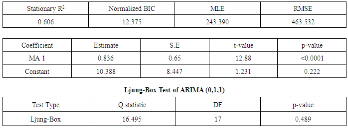
This model is a special case of ARIMA model, which is called an Integrated Moving Average Model.This model was diagnosed by Ljung-Box test and the p-value was quite large (greater than the usually chosen critical level of 0.05), the test is not significant and therefore we do not reject the null hypothesis, thus the residuals appear to be uncorrelated. This indicates that the residuals of the fitted ARIMA (0,1,1) model is a white noise, and for that reason, the model fit the series quite well, the parameter of the model are significant and the residuals are uncorrelated.The plots Fig 4 comprise of the time plot of the residuals, ACF plot of the residuals and the PACF plot of the residuals respectively. The time plots of the residuals clearly shows that the residuals appear to be randomly scattered, no evidence exists that the error terms are correlated with one another as well as no evidence of existence of an outlier. The residuals or errors are therefore conceived of as an independently identically distributed sequence with a constant variance and a zero mean. The ACF and the PACF plots of the residuals shows no evidence of a significant spike (the spikes are within the confidence limits) indicating that the residuals seems to be uncorrelated. Therefore, the ARIMA (0,1,1) model appears to fit well so we can use this model to make forecasts. This also shows that the residuals of ARIMA (0,1,1) model is a white noise process. Thus the residual plots corroborate the conclusion of the Ljung-Box test. 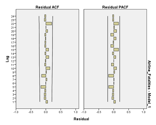 | Figure 4. Plot of Residual ACF and PACF of Airline Fatalities |
Table 4. ARIMA (0,1,1) Results
 |
| |
|
5. Forecasting with the Fitted Model
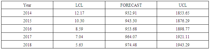
Thus, in time series modeling, researchers are motivated by the desire to produce a forecast with minimum error as possible. In this section, we assess the forecasting performance of Box-Jenkins models. The traditional Box-Jenkins approach is general and can handle effectively many time series encounter in reality.Forecasting the Major Airline Fatalities in the world using univariate Time Series Models, we computed one-step ahead forecasts for the fitted mode, i.e. ARIMA (0,1,1). These forecasts and their 95% confidence interval i.e. Lower confidence limit (LCL) and upper confident limit (ULC) for five years (i.e. 2014 – 2018) were summarized in Table 5, while Fig 5 depicts the observed and forecast plots of Major Airline Fatalities in the world, the values of the forecasts shows that occurrences of airline Fatalities will increase insignificantly for the next five years.  | Figure 5. The plot of the observed and forecast value of Airline Fatalities |
Table 5. Forecasts results with the Fitted ARIMA (0,1,1) Model
 |
| |
|
6. Conclusions
This research fit a univariate time series model to the major Airline Fatalities in the world from 1920 through 2013, the evaluation of pattern revealed that occurrence of Airline Fatalities were not constant but rather varied from one year to the other with no systematically visible pattern. The Box-Jenkins Autoregressive Integrated Moving Average (ARIMA) model was estimated and the best fitting ARIMA model was used to obtain the post-sample forecasts for five years. The fitted model was ARIMA (0,1,1) with Normalized Bayesian Information Criteria (BIC) of 3.014, Stationary R2 of 0.296, and Maximum Likelihood (MLE) estimate of 243.390, the mathematical equation of the fitted model was | (5) |
This model was further validated by Ljung-Box test with no significant Autocorrelation between the residuals at different lag times and subsequently by white noise of residuals from the diagnostic checks performed which clearly portray randomness of the standard error of the residuals, no significant spike in the residual plots of ACF and PACF. The fitted model was used to obtain the post-sample forecast for five years, we assessed the forecasting performance of Box-Jenkins models, we computed one-step ahead forecasts for the fitted mode, i.e. ARIMA (0,1,1). These forecasts and their 95% confidence interval i.e. Lower confidence limit (LCL) and upper confident limit (ULC) for five years (i.e. 2014 – 2018) indicates that Airline Fatalities will increase insignificantly for the next five years (2014-2018).
References
| [1] | Borenstein, Severin and Martin B. Zimmerman (1988). Market incentives for safe commercial airline operation. “ American Economic Review” 78: 913-35. |
| [2] | Bosh, Jean Claude, Woody W, Eckard, and Vijay Singal (1998). The competitive impact of air. |
| [3] | Box, G.E.P, and D.A. Pierce (1970). “Distribution of Residual Autocorrelation in Autoregressive-Integrated Moving Average Models”. J. American Stat. Assoc. 65: 1509-26. |
| [4] | Box, G.E.P, and G.M. Jenkins (1976). Time series analysis: Forecasting and control. Rev.ed. San Francisco. Holden-Day. |
| [5] | Hamilton, J. D. (1994), Time Series Analysis. Princeton University Press, New Jersey, USA. |
| [6] | Ljung G. M, and G.E.P Box (1978). “On a measure of lack of fit in time series models”. Biometrika, 65:67-72. |
| [7] | Mitchell, Mark L., and Michel T. Maloney (1989). Crisis in the cockpit? The role of market forces in promoting air travel safety. |
| [8] | Mohammed A. Quddus (2008). Time series count data models. An empirical application to traffic accidents. |
| [9] | Rose, Nancy L (1992). Fear of flying? Economic analysis of Airline Safety. |
| [10] | Salau M.O. (1998). ARIMA modeling of Nigeria’s crude oil Export, AMSE, modeling, measurement and control. Vol.18. No.1, 1-20. |
| [11] | www.airdisasters.co.uk (2002). Major Airline Disasters involving commercial passengers Airline 1920-2002. |
 Abstract
 Reference
 Full-Text PDF
 Full-text HTML