Mo'oamin M. R. El-Hanjouri , Bashar S. Hamad
Department of Applied Statistics, Al-Azhar University - Gaza, Gaza, Palestine
Correspondence to: Bashar S. Hamad , Department of Applied Statistics, Al-Azhar University - Gaza, Gaza, Palestine.
| Email: |  |
Copyright © 2015 Scientific & Academic Publishing. All Rights Reserved.
Abstract
This research applied methods of multivariate statistical analysis, especially cluster analysis (CA) in order to recognize the disparity in the living standards for family among the Palestinian areas. The research results concluded that there is a convergence in living standards for family between two areas formed the first cluster of high living standards which are the urban of middle West Bank and the camp of middle West Bank, also there was a convergence of living standards for family among the seven areas formed the second cluster of middle living standards which are the urban of North West Bank, the camp of North West Bank, the rural of North West Bank, the urban of South West Bank, the camp of South West Bank, the rural of South West Bank and the rural of middle West Bank. In addition, there is a convergence of living standards for family among the three areas formed the third cluster of low living standards which are the urban of Gaza strip, the rural of Gaza strip and the camp of Gaza strip. After a comparison among several methods of cluster analysis through a cluster validation (Hierarchical Cluster Analysis, K-means Clustering and K-medoids Clustering), the preference was for the Hierarchical Cluster Analysis method. However, after an examination to choose the best method of connection through agglomerate coefficient in the Hierarchical Cluster Analysis (Single linkage method, Complete linkage method, Average linkage method and Ward linkage method), the preference was for Ward linkage method which has been selected to be used in the classification. Moreover, the Discriminant Analysis method (DA) applied to distinguish the variables that contribute significantly to this disparity among families inside Palestinian areas and the results show that the variables of monthly Income, assistance, agricultural land, animal holdings, total expenditure, imputed rent, remittances and non-consumption expenditure are significantly contributed to disparity. Keywords Cluster Analysis (CA), Hierarchical Cluster Analysis (HCA), Discriminant Analysis (DA)
Keywords: Cluster Analysis (CA), Hierarchical Cluster Analysis (HCA), Discriminant Analysis (DA)
Cite this paper: Mo'oamin M. R. El-Hanjouri , Bashar S. Hamad , Using Cluster Analysis and Discriminant Analysis Methods in Classification with Application on Standard of Living Family in Palestinian Areas, International Journal of Statistics and Applications, Vol. 5 No. 5, 2015, pp. 213-222. doi: 10.5923/j.statistics.20150505.05.
1. Introduction
The living standards of family studies has been considered as one of the most important issues around the world. The distribution of income among families shows the extent of justice enjoyed by the community, the importance of economic development is not only the development of the national income but also the importance of the good distribution of income among families. The possibility of increasing national income and not increasing majority of family incomes leading to discontent of communities and not to well-being. The main purpose of the economic and political systems within the societies is to raise the standards of living for the majority of the population in the community by rational utilization of available natural and human resources in order to achieve balanced growth in all fields, and distributed equitable to the maximum possible extent, and while spreading phenomenon of inequality and recede centrist categories must be a serious interference by the government to limit this phenomenon and try to minimize the differences among social classes through the use of sound economic policies (Ahmed, 2010). In this study, the Palestinian areas have been divided into 12 area as follows (the urban of North West Bank, the rural of North West Bank, the camp of North West Bank, the urban of South West Bank, the rural of South West Bank, the camp of South West Bank, the urban of Middle West Bank, the rural of Middle West Bank, the camp of Middle West Bank, the urban of Gaza Strip, the rural of Gaza Strip, the camp of Gaza Strip). Moreover, this study applied multivariate statistical analysis techniques and method of multivariate cluster analysis in order to find out the disparity in standards of living family among the Palestinian areas, also used method of multivariate discriminant analysis to identify the factors that contribute significantly to this disparity between these families.
2. Study Problem
The study problem could be figured out through the disparity in standards of living family among the Palestinian areas using cluster analysis and identifying the variables that significantly contribute to the disparity among these families within these areas and the distinction among these sources using discriminant analysis. Briefly, “Estimating the number of data sets in the living standards of family in Palestinian areas using cluster analysis and the distinction among these totals using discriminant analysis”.
3. Objectives of Study
The major aim of this study is using multivariate cluster analysis in classification of Palestinian areas into homogeneous groups according to the standards of living for family and determines the extent of divergence and convergence between these areas and use multivariate discriminant analysis to identify the causing factors the discrepancy among these families within these areas. In addition, the following are some sub-objectives:• Application of cluster and discriminant analysis and explain the results of analyses together and mechanism of action statistically.• A comparison between a range of ways of clustering theoretically and practically.• To find the factors those affect the standard of living family and the study of the disparity among Palestinian areas
4. Source of Data
The data of this study has been taken from “The Palestinian Expenditure and Consumption Survey” that has been gathered by the Palestinian Central Bureau of Statistics (PCBS) in 2011. The aim of this survey is to study the expenditure and consumption for the family in the Palestinian society. This survey is executed nationwide yearly to study expenditure and consumption for the family.
5. Cluster Analysis Method
Cluster analysis (CA) is a set of tools for building groups (clusters) from multivariate data objects (Hardle & Simar, 2007), Cluster analysis is an important exploratory tool widely used in many areas such as biology, sociology, medicine and business (Yan, 2005), Cluster analysis is a multivariate method which aims to classify a sample of subjects (or objects) on the basis of a set of measured variables into a number of different groups such that similar subjects are placed in the same group (Cornish, 2007).The aim of this method is to construct groups with homogeneous properties out of heterogeneous large samples. The groups or clusters should be as homogeneous as possible and the differences among the various groups as large as possible. Cluster analysis can be divided into two fundamental steps: 1. Choice of a proximity measure: One checks each pair of observations (objects) for the similarity of their values. A similarity (proximity) measure is defined to measure the “closeness” of the objects. The “closer” they are, the more homogeneous they are.2. Choice of group-building algorithm: On the basis of the proximity measures the objects assigned to groups so that differences between groups become large and observations in a group become as close as possible (Hardle & Simar, 2007).
5.1. Basic Steps in Cluster Analysis
5.1.1. Element Selection
The purpose of cluster analysis is to explore the cluster structure in data without any prior knowledge about the true classification. The result is quite data-driven. In particular, the data structure will be defined by the elements selected for study. An ideal sample should represent the underlying clusters or populations. Inclusion of outliers (data points falling outside the general region of any cluster) should be avoided as much as possible so as to facilitate the recovery of distinct and reliable cluster structures, although they sometimes form a single cluster (Yan, 2005).
5.1.2. Variable Selection
Data investigated in cluster analysis are often recorded on multiple variables. The importance of choosing an appropriate set of variables for clustering is obvious. It is necessary to select enough variables to provide sufficient information about the underlying cluster structure. However, inclusion of unnecessary \noise "variable might \dramatically interfere with cluster recovery" (Milligan, 1996). Masking variables is De Soete's optimal weighting method, this method defines the distance between 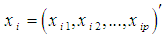 and as
 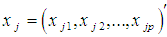 :
: Where wk; k = 1,…., p; are the optimal weights computed in a complex way so that the fit of the distance to an ultra metric matrix is optimized.Milligan (1989) showed that this method was effective in dealing with the masking problem, unfortunately didn't find the same favorable evidence for De Soete's method in their trials with different simulated data sets. Other attempts to solve this problem include different approaches to pursuing optimal variable weighting and variable selection strategies without weighting variables (Gnanadesikan et al., 1995).
5.1.3. Variable Standardization
Variable standardization may have striking impact on cluster analysis; the relative distances between pairs of objects may be changed after standardization, hence altering the cluster structure in the data. Although, standardization is usually suggested as an approach to making variables commensurate (Yan, 2005).
5.1.4. Distance Measure (Similarity/Dissimilarity)
The starting point of a cluster analysis is a data matrix with n measurements (objects) of p variables. The proximity (similarity) among objects is described by a matrix, the matrix D contains measures of similarity or dissimilarity among the n objects (Hardle & Simar, 2007).A basic assumption of cluster analysis is that objects assigned to the same cluster are closer (more similar) to each other than to those in other clusters. A large class of clustering techniques partition objects based on the dissimilarity matrix directly or indirectly (Yan, 2005).
5.1.5. Selection of Clustering Method
Choosing the clustering method should consider four aspects when selecting a method:First, the method should be designed to recover the cluster types suspected to be present in the data. Second, the clustering method should be effective at recovering the structures for which it was designed. Third, the method should be able to resist the presence of error in data. Finally, availability of computer software for performing the method is important (Yan, 2005).
5.1.6. Determining the Number of Clusters
There are no completely satisfactory methods that can be used for determining the number of population clusters for any type of cluster analysis. A fundamental problem in cluster analysis is to determine the number of clusters, which is usually taken as a prior in most clustering algorithms. Clustering solutions may vary as different numbers of clusters are specified. A clustering technique would most possibly recover the underlying cluster structure given a good estimate of the true number of clusters (Yan, 2005).It is tempting to consider the problem of determining "the right number of clusters" as akin to the problem of estimation of the complexity of a classifier, which depends on the complexity of the structure of the set of admissible rules, assuming the worst-case scenario for the structure of the dataset (Vapnik, 2006).
5.1.7. Interpretation, Validation and Replication
The process of evaluating the results of cluster analysis in a quantitative and objective way is called cluster validation (Dupes & Jain, 1988). It has four main components (Tan et al., 2005):(1) Determine whether there is non-random structure in the data. (2) Determine the number of clusters.(3) Evaluate how well a clustering solution fits the given data when the data is the only information available.(4) Evaluate how well a clustering solution agrees with partitions obtained based on other data sources. Among these, Component (3) is known as internal validation while Component (4) is referred to as external validation. Component (1) is fundamental for cluster analysis because almost every clustering algorithm will find clusters in a dataset, even if there is no cluster structure in it (Beglinger & Smith, 2001).
5.2. Hierarchical Cluster Analysis
Hierarchical techniques produce a nested sequence of partitions, with a single, all-inclusive cluster at the top and singleton clusters of individual points at the bottom. Each intermediate level can be viewed as combining two clusters from the next lower level (or splitting a cluster from the next higher level). The result of a hierarchical clustering algorithm can be graphically displayed as tree, called a dendogram.There are two basic approaches to generating a hierarchical clustering:a) Agglomerative Start with the points as individual clusters and, at each step, merge the most similar or closest pair of clusters. This requires a definition of cluster similarity or distance.b) Divisive Start with one, all-inclusive cluster and, at each step, split a cluster until only singleton clusters of individual points remain. In this case, we need to decide, at each step, which cluster to split and how to perform the split. (Dupes & jain, 1988) (Kaufman & Rousseeuw, 1990)
5.2.1. Agglomerative Algorithm Methods
Agglomerative procedures are probably the most widely used of the hierarchical methods. They produce a series of partitions of the data: the first consists of n single member ‘clusters’, the last consists of a single group containing all n individuals. Agglomerative algorithms are used quite frequently in practice. According to (Timm, 2002), the algorithm consists of the following step:1. Compute the distance matrix D = (d ij), i,j=1,...,n.2. Find two observations with the smallest distance and put them into one.3. Compute the distance matrix between the n −1 clusters.4. Find two clusters with the smallest inter cluster distance and join them.5. Repeat step 4 until all observations are combined in one cluster.
5.3. Non-Hierarchical Cluster Analysis
5.3.1. K-means Clustering Algorithm
k-means clustering is Partitional Clustering approach, k represents the number of clusters. The value of k is usually unknown a priori and has to be chosen by the user. Each cluster has a centroid, which is usually computed as the mean of the feature vectors in the cluster, the cluster membership of each data point under the k-means clustering algorithm is decided based on the cluster-centroid nearest to the point. As centroids cannot be directly calculated until clusters are formed, the user specifies k initial values for the centroids at the beginning of the clustering process. The actual centroid values are calculated once clusters have been formed (Shen, 2007).
5.3.2. K-mediods Clustering Algorithm
The k-medoids algorithm is a clustering algorithm related to the k-means algorithm and the medoid shift algorithm. Both the k-means and k-medoids algorithms are partitional (breaking the dataset up into groups) and both attempt to minimize squared error, the distance between points labeled to be in a cluster and a point designated as the center of that cluster. In contrast to the k-means algorithm, k-medoids chooses data points as centers (medoids or exemplars).K-medoids is also a partitioning technique of clustering that clusters the data set of n objects into k clusters with k known a priori. A useful tool for determining k is the silhouette.It could be more robust to noise and outliers as compared to k-means because it minimizes a sum of general pairwise dissimilarities instead of a sum of squared Euclidean distances. The possible choice of the dissimilarity function is very rich but in our applet we used the squared Euclidean distance (Mirkes, 2011).
5.4. Cluster Validation
The process of evaluating the results of cluster analysis in a quantitative and objective way is called cluster validation (Dupes & Jain, 1988). It has four main components (Tan et al., 2006):1- Determine whether there is non-random structure in the data. 2- Determine the number of clusters.3- Evaluate how well a clustering solution fits the given data when the data is the only information available.4- Evaluate how well a clustering solution agrees with partitions obtained based on other data sources. Among these, Component (3) is known as internal validation while Component (4) is referred to as external validation. Component (1) is fundamental for cluster analysis because almost every clustering algorithm will find clusters in a dataset, even if there is no cluster structure in it (Beglinger & Smith, 2001).
6. Discriminant Analysis Method
Discriminant Analysis (DA) a multivariate statistical technique used to build a predictive / descriptive model of group discrimination based on observed predictor --variables and to classify each observation into one of the groups, that allows one to understand the differences of objects between two or more groups with respect to several variables simultaneously. It is the first multivariate statistical classification method used for decades by researchers and practitioners in developing classification models, In DA multiple quantitative attributives are used to discriminate single classification variable. DA is different from the cluster analysis and the multivariate analysis of variance (MANOVA). It is different from the cluster analysis because prior knowledge of the classes, usually in the form of a sample from each class is required (Fernandez, 2002) (Hamid, 2010). The basic purpose of discriminant analysis is to estimate the relationship between a single categorical dependent variable and a set of quantitative independent variables.
7. Empirical Case Study
In this study will be used cluster analysis to classify Palestinian areas according to the standard of living for the family, the dependent variable is Palestinian areas which is divided into 12 regions, and will find a variable represents the standard of living of the regions will be used in a discriminant analysis. And then use the discriminant analysis to discriminate families within these areas and know the variables that affect the living standards of the regions and the dependent variable is the variable output of the cluster analysis, which represents the living standards of the areas.
7.1. Descriptive of the Data
The data consists of 11 variables (Monthly Income, Assistance, Monthly rent, Agricural land, Animal holdings, TOT_Cons, Tot_Exp, Imputed rent, Remittances, Taxes, non-consumption expenditure).Expenditure (Tot_Exp): It refers to the amount of Cash spent on purchase of goods and services for living purposes, and the value of goods and services payments or part of payments received from the employer, and Cash expenditure spent as taxes (non-commercial or non-industrial), gifts, contributions, interests on debts and other non-consumption items.Consumption (Tot_Cons) : It refers to the amount of Cash spent on purchase of goods and services for living purposes, and The value of goods and service payments or part of payments received from the employer, and own-produced goods and food, including consumed quantities during the recording period, and Imputed rent for own housing.Monthly Income: Cash or in kind revenues for individual or household within a period of month.Non-consumption expenditure: Interests on loans, fees and taxes.Animal holdings: The household have animal holdings (Cattle, Sheep and Goats, Poultry, Horses and Mules, Beehives).Agricural land: The household have agricural land. Taxes: Includes data about cash and in kind taxes which paid from household.Assistances: Includes data about cash and in kind assistances (assistance value, assistance source), also collecting data about household situation, and the procedures to cover expenses.Remittances: Includes data about cash and in kind remittances (remittances value, remittances source), also collecting data about household situation, and the procedures to cover expenses. Imputed rent: Value of imputed rent for house hold in Isrealian ShekelMonthly rent: Value of monthly rent for house hold which paid in Isrealian Shekel
7.2. The Application of Cluster Analysis
7.2.1. Using HCA to Classify
Our data areas Palestinian consist from 12 observations so that the suitable algorithm for estimating the number of clusters is hclust() where we used the agglomerative hierarchal clustering which begins with every case being a cluster. Similar clusters are merged and we can choose the number of clusters that maximizes the height at hierarchal cluster dendogram.
7.2.1.1. Similarity Measures
We will use the dist () function to calculate the distance between every pair of objects in a data set. There are many ways to calculate this distance information. By default, the dist () function calculates the Euclidean distance between objects however, we can specify one of several other options such as (Gower, Manhattan, Brary, Kulkulas)
7.2.1.2. Compares Dissimilarity Indices for Data
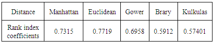
Use Rank correlations rankindex () between dissimilarity indices (Euclidean, Gower, Manhattan, Brary, Kulkulas).Table 1. Dissimilarity indices
 |
| |
|
The Euclidean distance is the best to measures dissimilarity.
7.2.1.3. Comparing Hierarchical Clustering Results
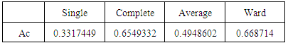
Agglomerative Coefficient (ac):Agnes() implements single, average , ward and complete linkage methods, it provides a coefficient measuring the amount of cluster structure, the agglomerative coefficient, where the summation is over all n objects, and mi is the ratio of the dissimilarity of the first cluster an object is merged to and the dissimilarity level of the final merge (after which only one cluster remains). Compare these numbers for four hierarchical clustering's of the data, are shown in table 2.Table 2. Agglomerative Coefficient
 |
| |
|
Ward linkage is doing the best job for these data, according to the agglomerative coefficient.
7.2.1.4. Determine Number of Cluster in Hierarchical Cluster Analysis
Looking at Figure 1. we notice that each object cluster with itself so we have 12 clusters. If we moved steps from down to upper we can notice that the U Middle WB and C Middle WB in one cluster with height = 4. The first cluster are agglomerate in another cluster with height=10. In second cluster that the R GAZA is in one cluster, U GAZA and C GAZA in another cluster. These two clusters are agglomerate in another cluster with height = 4. These two clusters are agglomerate in another cluster with height = 8.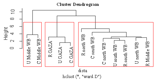 | Figure 1. Ward clustering among areas |
In third cluster R Middle WB and U North WB in one cluster and R South WB and U South WB and C North WB in another cluster. The clusters are agglomerate in a cluster with height = 3; and both clusters are agglomerate with C South WB with height = 4; and R North WB agglomerate with a cluster with height = 5; second and third cluster agglomerate with height = 8 and Both cluster are agglomerate with first cluster with height = 10. Simply displaying the group memberships isn't that revealing. A good first step is to use the table function to see how many observations are in each cluster. We'd like a solution where there aren't too many clusters with just a few observations, because it may make it difficult to interpret our results. The distribution among the clusters looks good.
7.2.2. Using K-Means Clustering
The k-means algorithm is very simple and basically consists of two steps. It is initialized by a random choice of cluster centers.
7.2.2.1. Determine the Number of Clusters in K Means?
We use Calinsky criterion these approach to diagnosing how many clusters suit the data.The Figure (2) is represent the number of cluster suit the areas data, the red point represent the correct number of clusters in 3.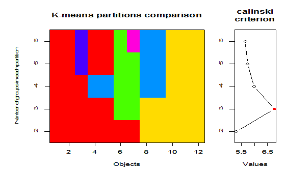 | Figure 2. Calinsky criterion approach |
The Figure (3) shows that there are three clusters. The first is in circle shape 1, the other with a circle shape 2, and the other with horizontal lines 3 and there is a distance separating them.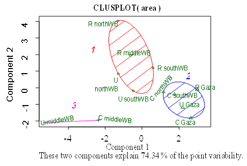 | Figure 3. Clust plot for the k-means clustering of the data |
7.2.3. Using K-Medoids Clustering
In k-means, cluster centers are given by the mean coordinates of the objects in that cluster. Since averages are very sensitive to outlying observations, the clustering may be dominated by a few objects, and the interpretation may be difficult. One way to resolve this is to assess clustering's with more groups expected: the outliers may end up in a cluster of their own. A more practical alternative would be to use a more robust algorithm where the influence of outliers is diminished, An overall measure of clustering quality can be obtained by averaging all silhouette widths. This is an easy way to decide on the most appropriate number of clusters.Figure (4): Silhouette plot for the k-medoids clustering of the data. The three clusters contain 5, 2 and 5 objects, and have average silhouette widths of 0.27, 0.23 and 0.42, respectively, The average silhouette width for this data set equals 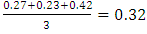 .
.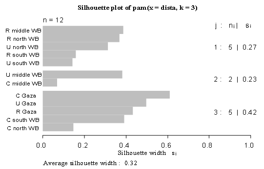 | Figure 4. Silhouette plot for the k-medoids clustering of the data |
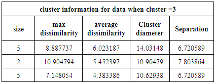
Table 3. above shows that there are 3 clusters containing 12 observations, One of them includes 5 observations with a maximum dissimilarity between them and a medoid equals 8.88. The diameter of the cluster equals 14.03 and the separation is 6.7, The second includes 2 observations with a maximum dissimilarity between them and a medoid equals 10.90, The diameter of the cluster equals 10.94 and the separation is 7.8, The third includes 5 observations with a maximum dissimilarity between them and a medoid equals 7.14, The diameter of the cluster equals 10.6 and the separation is 6.7.Table 3. Cluster information for data
 |
| |
|
Note:In general, the structure of cluster is weak and not acceptable in the 2nd cluster because of the available variables and inability of adding another variables due to unavailability of these variables within the census.
7.2.4 Cluster Validation
7.2.4.1 Internal Validation
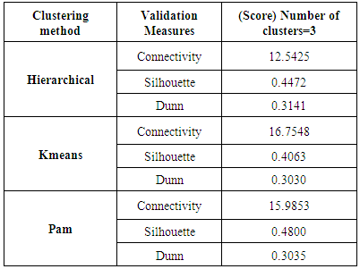
The internal validation measures are the connectivity, Silhouette Width, and Dunn Index. The neighborhood size for the connectivity is set to 10 by default.Hierarchical clustering with three clusters performs the best in (Connective, Dunn) while the Pam is the best in (Silhouette). Recall that the connectivity should be minimized, while both the Dunn Index and the Silhouette Width should be maximized. Thus, it appears that Hierarchical clustering outperforms the other clustering algorithms under each validation measure.Table 4. Compare between internal validation measures
 |
| |
|
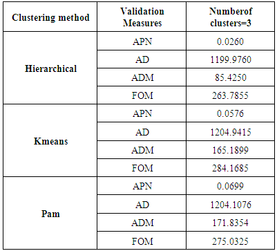
7.2.4.2. Stability Validation
The stability measures include the APN, AD, ADM, and FOM. The measures should be minimized in each case. Stability validation requires more time than internal validation, since clustering needs to be redone for each of the datasets with a single column removed.For the all measures, Hierarchical clustering with three clusters again gives the best score. Therefore, hierarchical clustering with three clusters has the best score in all cases.
7.3. Application of Discriminant Analysis
Discriminant analysis has been widely used in similar studies and applied on different topics in different countries of the world.The object of Discriminant analysis those classify the families inside Palestinian areas according living standard on account of results of cluster analysis, Were found discriminant analysis based on the three groups drawn from the results of cluster analysis were placed observations of first cluster (U Middle WB, C Middle WB) represent High living standard in the first group have also been placed observations of second cluster (U South WB, C South WB, R South WB, R North WB, C North WB, U North WB, R Middle WB) represent Middle living standard in the second set as well as the observations that have been placed third cluster (R Gaza, C Gaza, U Gaza) in the third set, when the discriminant analysis, the dependent variable is based on the three groups and so was the use of discriminant analysis in the case of more than two groups (three groups) and the results are shown below:
7.3.1. Test of Multivariate Normality
Often, before doing any statistical modeling, it is crucial to verify whether the data at hand satisfy the underlying distribution assumptions. Multivariate normal distribution is one of the most frequently made distributional assumptions when using multivariate statistical techniques.Also, from an important property of multivariate normal distribution, we know that if X=(X1,X2,….,Xp) follow the multivariate normal distribution, then its individual components X1,X2,…..,Xp are all normally distributed. Therefore, we need to examine normality of each Xi to guarantee that X=(X1,X2,…,Xp) is multivariate normal distributed.Here, we use quantile-quantile plot (QQ plot) to assess normality of data though there are more formal mathematical assessment methods. The reason is that with a large dataset, formal test can detect even mild deviations from normality which actually we may accept due to the large sample size. However, a graphical method is easier to interpret and also have the benefit to easily identify the outliers. In QQ plot, we compare the real standardized values of the variables against the standard normal distribution. The correlation between the sample data and normal quantiles will measure how well the data is modeled by a normal distribution. For normal data, the points plotted should fall approximately on a straight line in the QQ plot. If not, data transformation like logarithm and square root transformation can be applied to make the data appear to be more closely normally distributed.We used different forms of transformation on the variables to obtain the substitute variables which perform better on normality, such as (log(log(Assistance), log(log(Monthly rent), log(Monthly Income), log(TOT_Cons), log(log(Tot_Exp)), log(Non-consumption expenditure), log(log(Taxes)), Sqrt(log(Remittances)), log(Imputed rent)).
7.3.2. Test for Covariance Matrix Equality
The second is that the covariance matrices are equal. Box's M test is used to see if another assumption of LDA holds: are the covariance matrices equal or not? The null hypothesis is that they are, the alternative hypothesis is that they are not.Another assumption is that the variables should not be highly correlated. The correlation coefficient between each pair of variables should be calculated.Box's M test testing the assumption of equal covariance for equality of the group covariance matrices. In this case, Box's M statistic had a value of 2255.935 with a probability of 0.00. Since the result is significant (p < 0.05) so there is sufficient evidence that we reject the hypothesis that the groups covariance matrices are equal.
7.3.3. Test the Significance of the Model
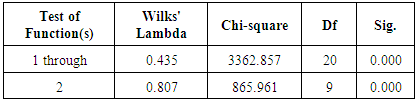
To test the significance of the model as a whole, we have the following two hypotheses: - Null hypothesis: the three groups have the same mean discriminant function scores; H0: μ1= μ2 =μ3- Alternate hypothesis: HA: μ1, μ2, μ3 at least of them are not equal.Table (5) shows that the value of wilks' lambda statistic for the test of function 1 through 2 functions (chi-square =3362.857) has probability of 0.000 which is less than or equal to the level of significance of 0.05.Table 5. Compare between Stability validation measures
 |
| |
|
After removing function 1, the wilks' lambda statistic for the test of function 2 (chi-square = 865.961) has a probability of 0.000 which is less than the level of significance of 0.05. The significance of the maximum possible number of discriminant functions supports the interpretation of a solution using 2 discriminant functions. That is the null hypothesis is rejected and the model differentiates scores among the groups significantly.
7.3.4. The Function
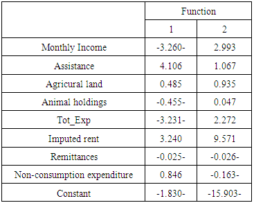
The main objective of this study is to estimate a discriminant function to estimate the expected family according to standard deviation in Palestinian areas.The table (6) shows the coefficients of the variables in the standardized discriminant function. The coefficients are the multiplier of the variables when they are in original measurement units. By using the variables and the coefficients, the equation is often known as discriminator.Table 6. Wilks' Lambda Test
 |
| |
|
The table Contains the Unstandardized discriminant coefficients. These would be used like unstandardized b which is -1.830 for function 1 and -15.903 for function 2, they are used to construct the actual prediction equation which can be used to classify new casesD1 = - 1.830 – 3.260 + 4.106 + 0.485 (Agricural land) - 0.455 (Animal holdings) – 3.231 + 3.240 – 0.025 + 0.846)D2 = -15.903 + 2.993 + 1.067 + 0.935 (Agricural land) + 0.047 (Animal holdings) + 2.272 + 9.571 – 0.026 - 0.163)
7.3.5. Assessing the Validity of the Model
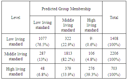
In order to check the validity of the model and to know the accurate forecasting power of the estimated model, at this stage, will look at the classification /prediction / confusion matrix. The matrix is constructed based on the prediction of the analysis sample by the estimated model and presented by the table (7).Table 7. Canonical Discriminant Function Coefficients (Unstandardized Coefficients)
 |
| |
|
The primal diagonal of the matrix presents the accuracy rate on the model and the off diagonal of the matrix presents the misclassification rate of the estimated model. The first element of the primal diagonal presents the rate-a case is actually in group 1 and the estimated model forecasted as group 1 divided by the number of the cases in group 1 and the rate is 76.5 percent. The second element of the primal diagonal presents the rate-a case is actually in group 2 and the estimated model forecasted the case as group 2 divided by the number of cases in group 2 and the rate is 82.2 per cent. The Third element of the primal diagonal presents the rate-a case is actually in group 3 and the estimated model forecasted the case as group 3 divided by the number of cases in group 3 and the rate is 39.3 per cent The total of the primal diagonal divided by the total number of the cases in the analysis sample is equal to correct prediction rate which is also known as hit ratio.Table 8. Classification Results
 |
| |
|
8. Conclusions
The following is the most important conclusions of this study:1. We used agglomerative hierarchical cluster analysis to classify Palestinian area's into clusters,a) we conducted a comparison between the four methods to calculate the dissimilarity matrix: Euclidean distance, Gower distance, Kulkulas distance and Brary distance, using technique (Rand index Coefficient) in order to achieve to the best method that calculate the distance, the Euclidean distance is the best method to measures similarity.b) We conducted a comparison between the four methods to choose the best linkage method: Single linkage Agglomerative Clustering, complete linkage Agglomerative Clustering, Average Agglomerative Clustering and Ward’s Minimum Variance Clustering, using technique (Agglomerative Coefficient) in order to achieve to the best clustering method, The Ward linkage is doing the best job for these data.c) Transformed the Palestinian's areas into three groups using agglomerate ward clustering method.2. To confirm with results we conducted a comparison among the three clustering method: hierarchal clustering method, k-means clustering and k-mediods clustering, using cluster validation technique that contain (internal validation, stability validation) in order to achieve to the best method that represent the data. Hierarchical clustering with three clusters performs the best in internal validation measures and stability validation measures.3. Took observations of the three groups as a dependent variable and use the discriminant analysis for the classification of observations that belong to one of the three groups.4. Correct classification rate is 73.3%, which that families are classified correctly that 3317 out of 4317 families had correctly classified to group to which they belong.
References
| [1] | Ahmed A. Y. (2010), "Analyse and measure well-being and their relationship to the justice the distribution of income In the city Kirkuk for the year 2009", Management and Economics Journal (83):278-307. |
| [2] | Fernandez C. G. (2002), “Discriminant Analysis, A Powerful Classification Technique in Data Mining” Department of Applied Economics and Statistics ,University of Nevada, Reno, journal of Statistics and Data Analysis ,paper 247- 27. |
| [3] | Cornish R. (2007) "Introduction to Cluster analysis, and how to apply it using SPSS " MLSC, Loughborough University. |
| [4] | Härdle W., Simar L. (2007), "Applied Multivariate Statistical Analysis", 2-edition, Berlin, Germany. |
| [5] | Hamid, Hashibah. (2010). "A New Approach for Classifying Large Number of Mixed Variables". World Academy of Science, Engineering and Technology. |
| [6] | Olugboyega M. O. (2010), “Loans and advances evaluation with discriminant analysis”, Department of Statistic, Nnamdi Azikiw University, Awka. |
| [7] | Savić M., Brcanov D., Dakić S. (2008) “Discriminant Analysis Applications and Software Support”, Management Information Systems, Vol. 3, No. 1, pp. 029-033. |
| [8] | Timm Neil H. (2002). "Applied Multivariate Analysis", Springer- Verlag New York, Inc.Usa. |
| [9] | Robert B. , Richard B. (2009), “Business Research Methods and Statistics using SPSS”, North America, California |
| [10] | Yan M., (2005), "Methods of Determining the Number of Clusters in a Data Set and a New Clustering Criterion", Ph.D Thesis in Philosophy in Statistics, Faculty of the Virginia Polytechnic , Institute and State University, Blacksburg, Virginia |
| [11] | Shen J. (2007), "Using Cluster Analysis, Cluster Validation, and Consensus Clustering to Identify Subtypes of Pervasive Developmental Disorders", M.Sc. in Science, Queen's University, Ontario, Canada. |
| [12] | Guesv P. (2005), "Models of Credit Risk for Emerging Markets", Master Thesis in Industrial and Financial Economics ,School of Business, Economics and Law, Goteborg University. |
| [13] | Abdi, H. (2007), "Encyclopedia of measurement and statistics". Thousand oak(CA) sage, 270-275.[Retrieved October 15, 2014 from http : //www.ut dallas.edu]. |
| [14] | Beglinger L. J., Smith T. H. (2001)"A Review of Subtyping in Autism and Proposed Dimensional Classification Model." Journal of Autism and Developmental Disorders. 31(4): 411-22. |
| [15] | Mirkes E.M. (2011), "K-means and K-medoids applet". University of Leicester , http://www.math.le.ac.uk/. |
| [16] | Tan P. N., Steinbach M., Kumar V., (2006) "Introduction to Data Mining", Michigan State University, University of Minnesota. |
| [17] | Dubes C. R. & Jain K.A.(1988), "Algorithms for Clustering Data", Prentice Hall |
| [18] | Milligan G. W. (1989) "A validation study of a variable weighting algorithm for cluster analysis", Journal of Classification, 6: 53-71. |
| [19] | Gnanadesikan R., Kettenring J. R, and Tsao S. L. (1995) "Weighting and selection of variables for cluster analysis". Journal of Classification, 12:113-136. |
| [20] | Vapnik V. (2006) "Estimation of Dependences Based on Empirical Data ", Springer Science + Business Media Inc., 2d edition. |
| [21] | Tan P. N., Steinbach M., Kumar V. (2005) "Introduction to Data Mining". Pearson Addison Wesley. |
| [22] | Kaufman L. and Rousseeuw P. J., (1990) "Finding Groups in Data: an Introduction to Cluster Analysis ", John Wiley and Sons. |
 Abstract
 Reference
 Full-Text PDF
 Full-text HTML