Smart A. Sarpong 1, Seungyoung OH 2, Richard K. Avuglah 3, N. N. N. Nsowah-Nuamah 4, Youngjo Lee 2
1School of Graduate Studies, Research and Innovation, Kumasi Polytechnic, Ghana
2Department of Statistics, Seoul National University, South Korea
3Department of Mathematics, Kwame Nkrumah University of Science and Technology, Kumasi, Ghana
4Rector, Kumasi Polytechnic, Ghana
Correspondence to: Smart A. Sarpong , School of Graduate Studies, Research and Innovation, Kumasi Polytechnic, Ghana.
| Email: |  |
Copyright © 2015 Scientific & Academic Publishing. All Rights Reserved.
Abstract
Dissimilar characteristics in individual location treatment effects can be modelled as a random effect in a community of many and different individual observations. This study demonstrates the excellent performance of higher levels and very recent extensions of the Generalized Linear Mixed Models (GLMM); Hierarchical Generalized Linear Models (HGLM) in the global quest to developing Statistical Models with highest model accuracy. The analyses is based on raw data available at the regional Monitoring and Evaluation office of the Linking Farmers to Markets (FtM) project in Tamale - Ghana. Physical support (Fixed effect) variables measured include; crop type, Financial Credit, Training, Study tour, Demonstrative Practical’s, Networking Events, Post-harvest Equipment, Number of farmers in the FBO and Plot size cultivated. Dependent variable measured is Total Crop Yield whereas the regions and the particular communities were treated as random variables. Results showed that the HGLM 2 had the ability of specifying different suitable fixed effects model from a known distribution, a random effects model allowed to follow conjugates of arbitrary distributions from the GLM family and a dispersion model. We conclude that the HGLM 2 performs far better, gives a more fitting models and improves the quality of the crop yield models significantly.
Keywords:
HGLM, GLM, Crop yield, H-Likelihood, Profile-Likelihood, Random-Effects
Cite this paper: Smart A. Sarpong , Seungyoung OH , Richard K. Avuglah , N. N. N. Nsowah-Nuamah , Youngjo Lee , Analysis of Crop Yield Physical Support Services Data Using Hierarchical Generalized Linear Models, International Journal of Statistics and Applications, Vol. 5 No. 5, 2015, pp. 196-207. doi: 10.5923/j.statistics.20150505.03.
1. Introduction
Ghana’s agro-ecological zones have significantly different agricultural structure and corresponding difference in the regional distributions of her agricultural GDP. These regional differences have important effects for sub-sector level agricultural growth strategies. The Forest Zone continuous to be the highest producer of major agricultural products, accounting for 43 per cent of agricultural GDP, as compared to about 10 per cent in the Coastal Zone, and 26.5 per cent and 20.5 per cent in the Southern and Northern Savannah Zones, respectively (Breisinger et al. 2008). The principal producer of cereals and livestock is the Northern Savannah zone. More than 70 per cent of the country’s sorghum, maize, millet, cowpeas, groundnuts, beef and soybeans come from the Northern Zone, while a large share of higher-value products, such as cocoa and livestock (mainly commercial poultry) is supplied by the Forest Zone.There are also indications of different agricultural income structures due to the heterogeneous agricultural production structure across all the regions in Ghana. Almost half of agricultural income comes from two of Ghana’s major export goods (cocoa and timber) which are produced in the Forest Zone. Agricultural exports also plays a vital role in the total agricultural income for the Coast and Southern Savannah Zones. In contrast, 90 per cent of agricultural income in the Northern Zone comes from staple crops and livestock (World Bank Global Forum on Agriculture, 2010).As is the case in most developing countries, the Ghanaian government can only devote limited resources to agricultural extension programs and so most programs are only administered to a limited proportion of the population. Because there is significant variation of farm size throughout the three northern regions and Ghana as a whole, and likely significant variation in the determinants of output for different sized farms, it is critical for all stakeholders, the academia and the general public to understand which support services and policies will benefit farms and improve crop yield for the different farmer based organizations of different farm sizes in different locations throughout the three northern regions with application of the hierarchical generalized linear models (HGLMs) of Lee and Nelder (1996).Lee and Nelder (1996) developed the HGLMs from three commonly used existing model classes; generalized linear models (McCullagh and Nelder, 1989), linear mixed models having both fixed and random effects and models with structured dispersions as used in analysis for quality improvement (Lee and Nelder, 1998). The hierarchical generalized linear models (HGLMs) extends generalized linear models (GLMs) to include random components in the linear predictor with arbitrary distributions. It uses the h-likelihood (Lee and Nelder, 1996) for inference about fixed and random effects given dispersion components and an adjusted profile h-likelihood for inference about dispersion components given fixed and random effects. This method promotes reliable and useful estimators. It shares properties with those obtained from marginal likelihoods, while having the advantage of not requiring to integrate out the random effects.The hierarchical generalized linear models (HGLMs) include generalized linear mixed models (GLMMs), which have normal random components. The h-likelihood for inference results in an extension of likelihood inference, providing an efficient fitting algorithm for the various likelihood-ratio tests and systematic model-checking methods. The method leads to statistically reliable and efficient estimators (Lee Y, Nelder J. A., 2001) similar to those obtained from marginal likelihood, while having the considerable advantage of not requiring the integrating out of random-effects. Their h-likelihood method is an extension of classical likelihood inference, and so needs neither the use of prior probabilities nor computationally intensive methods such as Monte-Carlo Markov’s chain (MCMC).We fit in this paper an HGLM to a crop yield data, in which the heterogeneous Regional and Community effects are treated as random effects. In our analysis we suggests that a system of support services; Access to credit facility, Training, Study tour, Demonstrative practical, Networking events and Post-harvest Equipment’s, plays an important role in determining crop yields even though their individual and interaction effects on yield is not uniform across farmer base organizations. We focused mainly on the production of Maize and Soy beans in northern part of Ghana where there is substantial farming activity. Maize and Soy beans are the very much cultivated crops in these parts of the country due to their vegetation which supports the growth of grains and cereals. Beyond the numbers and descriptive statistics on yield of such crops, our primary aim is to fit an HGLM to the data. We seek to assess covariates or variables that significantly influences crop yield in the Northern regions of Ghana.Unobservable with names such as random effects, latent processes, factor, missing data, unobserved future observations, potential outcomes etc. appear in a number of statistical literatures. Handling of such unobservable is vital to new extended likelihood inferences. Without resorting to empirical Bayes frameworks, inferences can be obtained (Lee and Nelder, 2002). A single algorithm, iterative weighted least squares, can be applied in all new models and needs neither prior distributions of parameters nor multi-dimensional quadrature. The h-likelihood is extremely important in relation to synthesis of the computational algorithms required for this wide class of new models. The algorithm can be reduced to the fitting of two-dimensional set of generalized linear models with one dimension being the mean and dispersion, and the other being fixed and random effects. Hence, no special code is needed for the estimation of dispersion components. This formulation implies that, the model-checking techniques derived for generalized linear models (McCullagh and Nelder, 1989, chapter 12), can be carried over to these new class of models. The hierarchical generalized linear models method does not require the use of prior probabilities.Jiao H et.al (2005) in their article titled “Modelling local item dependence with the hierarchical generalized linear model”, proposes a three-level hierarchical generalized linear model (HGLM) to model local item dependence (LID). Their proposed three-level HGLM was examined by analyzing simulated data sets and was compared with the Rasch-equivalent two-level HGLM that ignores the nested structure of such test items. Their results demonstrated that the proposed model could capture LID and estimate its magnitude. Also, the two-level HGLM resulted in larger mean absolute differences between the true and the estimated item dependence than those from the proposed three-level HGLM. Furthermore, it was demonstrated that the proposed three-level HGLM estimated the ability distribution variance unaffected by the LID magnitude, while the two-level HGLM with no LID consideration increasingly underestimated the ability variance as the LID magnitude increased.HGLM for the analysis of lactation curves with heterogeneous residual variances versus time was used by Jaffrezic et al. (2000). Noh et al (2005) modeled heavy tailed distributions for random effects to take ascertainment into account in quantitative trait locus (QTL) studies. Noh et al. (2006a) used HGLM to reduce bias in heritability estimation for binary traits in human family data. HGLM was also utilized with random effects in survival analysis (Noh et al. 2006b). In recent times, the double hierarchical generalized linear models (DHGLM) has been used for fast variance component estimation in a model with genetic heterogeneity in the residual variance of an animal model (Ronnegard et al. 2010). DHGLM has also been suggested in the detection of variance-controlling QTL (Ronnegord and Valdar, 2010).
2. Method of HGLM
We begin with the well-known structure of GLMs in which observations  are assumed to have means
  and to be independently distributed with a distribution belonging to a one-parameter exponential family. The means
  are assumed to depend on a set of explanatory variables
  via a linear predictor
  and a link function
  , for some monotone function
  . A normal distribution for the errors together with an identity link function results in the classical regression model, the Poisson distribution with log link gives log-linear models, the binomial distribution with logit link gives logistic regression, and so on.The linear predictor in HGLMs is extended to include extra random components
  . This extended linear predictor
  is assumed to be related to
  , the conditional mean of
  given
given  , by a link function
  where
where  is the model matrix for the random effects. The random components
  in the linear predictor are assumed to be derived from the underlying random effects, by a one- to-one function
  . Assumptions about the distribution of u and the form of the function
  complete the specification. Two important subclasses of HGLMs are GLMMs and conjugate HGLMs. In GLMMs the
  are assumed normal, with
  , whereas in conjugate HGLMs the
  are assumed to follow the conjugate distribution to the conditional distribution of
  given
given  , with
  equal to the canonical link. An example of the latter is the binomial-beta HGLM, where
  has the beta distribution and contributes
  to the linear predictor. In both cases
  covers the whole of the real line, as is desirable in a component of the linear predictor. They overlap in the normal-normal HGLM. HGLMs form an extension of the Gaussian random-effect models to non-Gaussian distributions and provide, we believe, a unified, logical and flexible approach to meta-analysis.
2.1. H-likelihood
Estimation of the fixed effects of models with random effect by increasing the marginal likelihood, after integrating out the random effects, is broadly used. Relatively there exist no analytic form for the marginal likelihood. The same implies to beta-binomial models with non-null fixed effects. For HGLMs we use the h-likelihood, which consists of two parts: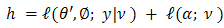 | (1) |
where  is the logarithm of the density function for
  with parameter
  , and
, and | (2) |
for  . As a result of the random effects
  not being observed, the second term is not of itself a traditional Fisherian likelihood; moreover, we affirm that the h-likelihood taken as a whole is the natural extension of Fisher likelihood to models with random components. If
 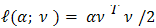 , that is, is proportional to the log-likelihood from
 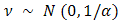 , the h-likelihood becomes Breslow and Claytons (Breslow N.E and Clayton D.G, 1993) penalized likelihood for a GLMM. Given the two dispersion components,
  in the
  distribution and
  in the
  distribution, we estimate
  simultaneously by increasing the h-likelihood. The h-likelihood provides a pivot for an extended version of the restricted (or residual) maximum likelihood estimation for
  of Patterson and Thompson (Patterson HD and Thomas R, 1971), applicable to all HGLMs. The resulting parameter estimators for
  are statistically reliable and efficient.
2.2. Model Checking
We believe that the importance of model checking after fitting random-effect models is insufficiently stressed. For GLM models, model-checking plots already exist (McCullagh P and Nelder J.A, 1989). The estimation methods for HGLMs can be reduced to fitting two interconnected GLMs and thus GLM model-checking method can also be utilized in checking for assumptions about HGLMs (Lee Y and Nelder J.A, 2001).
2.3. Checking the Distribution of y/v
We use two plots: the plot of the standardized deviance residuals against the fitted values  on the constant information scale (Lee and Nelder JA, 1996), and the plot of the absolute residuals for checking conditional distribution
  , besides normal probability plots. The two plots should show running means that are approximately straight and flat for them to be accepted as an adequate model. Marked curvatures in the first plot represents either inadequate link functions or missing terms in the linear predictor, or both. A satisfactory first plot means, the choice of variance function for
  , can be checked by the second plot. For instance, a down- ward marked trend by the second plot, means that the residuals are decreasing in absolute value as the mean increases, implying that the assumed variance function is increasing too fast with the mean. The running mean for trend is sensitive to the points at the extremes, so we concentrate on the central part of the graph. Outliers in the Normal probability plots usually accounts for Curvatures in the top two plots. These are primarily caused by the observations that take boundary values.
2.4. Checking the Distribution of 
An individual extreme random treatment trial interaction can be checked to be consistent or not with the rest, in relation to looking or not looking like the extreme value in a sample from a normal distribution. If it is inconsistent, a careful investigation of the various model assumptions, for instance the distributional assumption about  , may be necessary to accommodate it. If it turns out to not be a false outlier, it can be treated as a: fixed effect in order to remove its effects in estimating the other
  .
.
3. Results
3.1. Data Information
The analyses is based on raw data available at the regional Monitoring and Evaluation office of the Linking Farmers to Markets (FtM) project in Tamale - Ghana. The project is organized by the Alliance for a Green Revolution in Africa (AGRA) with the primary goal of easing the flow of produce from the farm-gate to the market by linking smallholder farmers to commercial buyers and processors. (FtM Grant Narrative Report, 2011).In all, data from 800 Maize & Soybean farmer based organizations (FBOs) were gathered by means of a structured questionnaire. This was later cleaned to 790 distinct observations. The Famer based organizations (FBOs) were randomly selected through a multi-stage random procedure. First, proportional randomizations resulted in selecting three (3) farming communities each from the Upper East and West regions while seven (7) were selected from the Northern Region.Fixed effect variables measured include; crop type (Maize or Soybean), Financial Credit (Acquired or Not), Training (Acquired or Not), Study tour (Acquired or Not), Demonstrative Practicals (Acquired or Not), Networking Events (Acquired or Not), Post-harvest Equipment (Acquired or Not), Number of farmers in the FBO and Plot size cultivated. Dependent variable measured is Total Crop Yield. The regions and the particular communities are treated as random effects. The target population consists of mainly Maize and Soybeans Farmer based organizations in selected communities in the three Northern regions of Ghana. Northern Region = 7 communities, Upper East Region = 3 communities, Upper West Region = 3 communities. Famer based organizations (FBO’s) interviewed = 800 with 10 missing data. Hence total FBO’s interviewed = 790.The R Statistical Analysis software (dhglmfit package) was used throughout the analysis in fitting the HGLM’s.
3.2. Exploratory Analysis
Firstly, the raw data is plotted and the patterns of Crop yield against some selected covariates are observed. Figure 3.1 presents the observed scatterplot of the crop yield against Plot size, Figure 3.2 presents the observed scatterplot of the crop yield against number of Farmers, and Figure 3.3 presents the observed scatterplot of the crop yield against Regions while figure 3.4 presents the observed scatterplot of the crop yield against the 13 communities.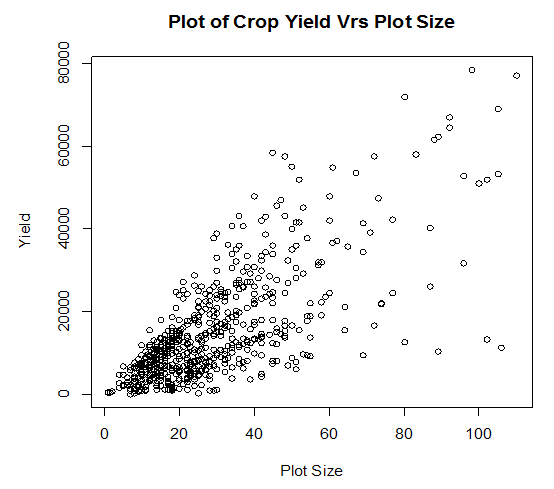 | Figure 3.1. Scatterplot of crop yield against Plot size |
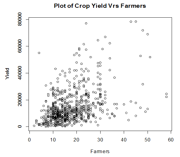 | Figure 3.2. Scatterplot of crop yield against number of famers |
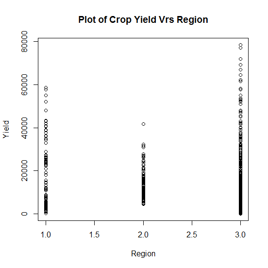 | Figure 3.3. Plot of crop yield against Regional locations |
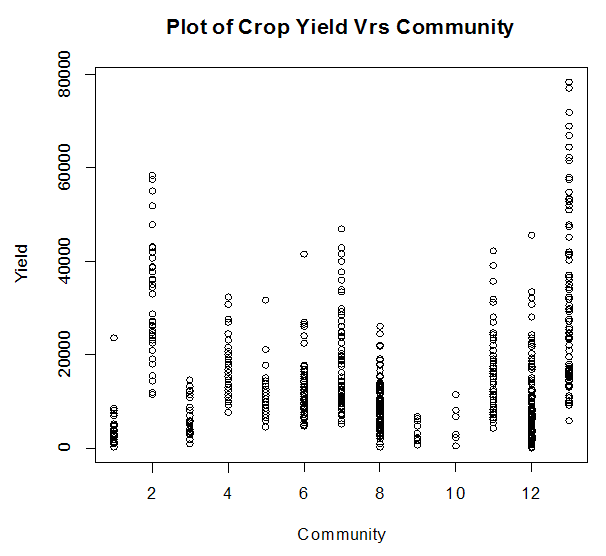 | Figure 3.4. Plot of crop yield against Communities |
3.3. Hierarchical Generalized Linear Models (HGLM 1)
Although in most instances, the normal distribution is expedient for assigning correlations in random effects, the use of other distributions for the random effects to a large extent enriches the class of models. Lee and Nelder (1996) extended GLMMs to hierarchical GLMs (HGLMs), referred to in this study as HGLM 1, in which the distribution of random components are extended to conjugates of arbitrary distributions from the GLM family. Figure 3.5 and 3.6 represent diagnostic plots for the Gaussian and Gamma HGLM’s respectively.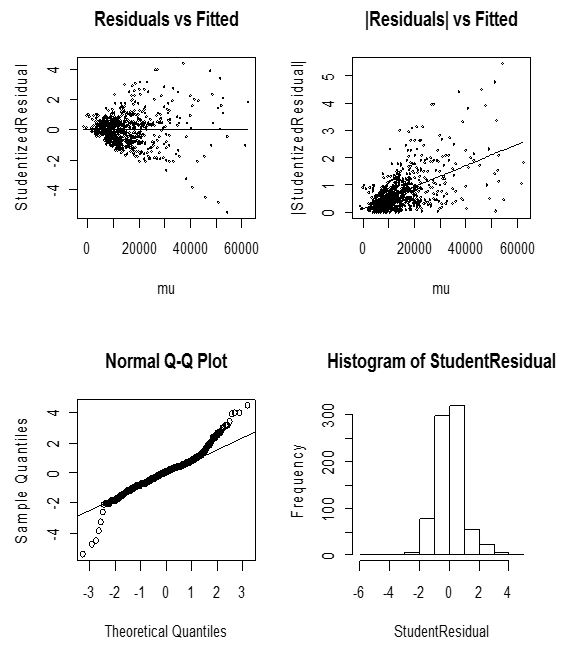 | Figure 3.5. Diagnostic plots of Gaussian HGLM 1 for crop yield |
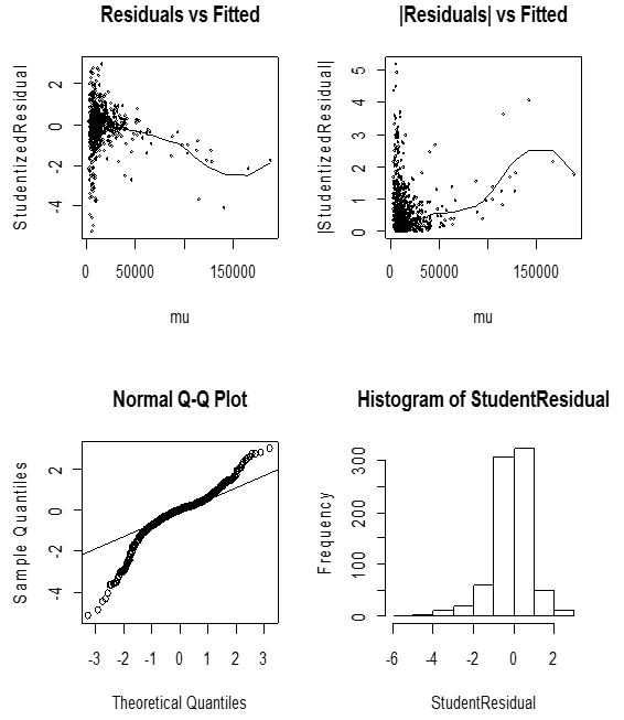
 | Figure 3.6. Diagnostic plots of Gamma HGLM 1 for crop yield |
The Gaussian diagnostic plots have some satisfactory features although not the best. The normal plot shows some discrepancy. Moreover, the histogram of residuals is almost symmetric. These are satisfactory indications of an appropriate model. We sort to remove any likely defects by extending to an HGLM with gamma errors and a log link. The model-checking plots does not come out appreciably as compared to the Gaussian model. Figure 3.6 shows the resulting plots.
3.3.1. Model Interpretation and Discussion
Table 1 represents the model parameter estimates for both the Gaussian and the Gamma HGLM’s.  or
or  on the table represents the mean model. Considering the random effects of Regions and the specific farming communities, the final mean model for the Gaussian HGLM does not include access to credit, Study tour, demonstrative practical’s, Networking events and post-harvest equipment’s. In the counterpart model for the Gamma HGLM, only number of farmers and the cultivated plot size were significant contributors to crop yield when the random effects of Regions and the specific farming communities are considered in the model.
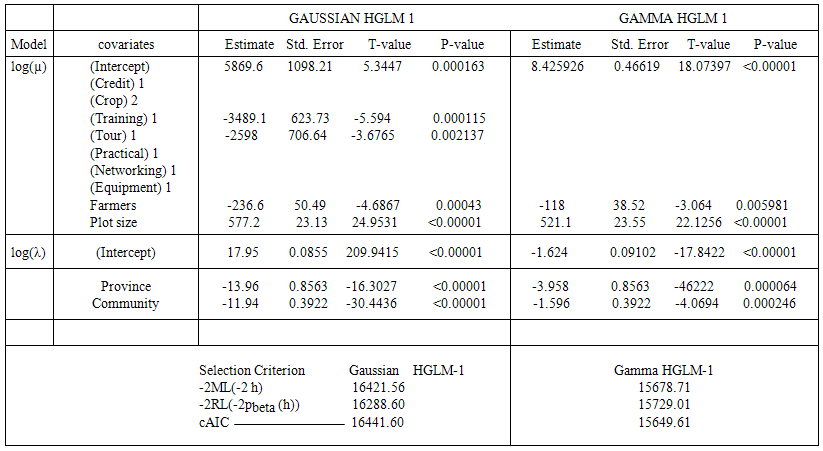 | Table 1. Comparative Model Estimates for Gaussian HGLM and Gamma HGLM |
3.4. Hierarchical Generalized Linear Models (HGLM 2)
HGLM 2 is an extension of the above discussed Hierarchical Generalized model (HGLM 1). It is useful in modeling sparse discrepancies as being caused by variation in the dispersion, and to look for covariates that may explain them with the help of the techniques of joint modelling of mean and dispersion (Lee and Nelder, 2002). With the success stories of the HGLM (Lee and Nelder, 2002), there was the need to extend the HGLM to enable models with structured dispersion as used in the analysis data from quality improvement experiments (Lee and Nelder 1998). HGLM 2 therefore comprises of a fixed effects model from a known distribution, a random effects model allowed to follow conjugates of arbitrary distributions from the GLM family and a dispersion model. Figures 3.7 and 3.8 represents the diagnostic plots for the Gaussian and Gamma H-GLM’s (2) respectively.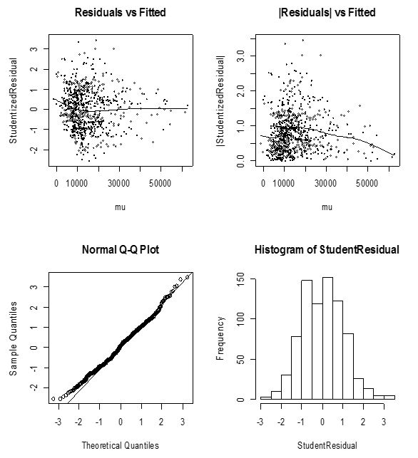 | Figure 3.7. Diagnostic plots of Gaussian HGLM 2 for crop yield |
 | Figure 3.8. Diagnostic plots of Gamma HGLM 2 for crop yield |
From figure 3.7 the diagnostic plots have several excellent features compared to the Gaussian HGLM (1) diagnostic plots in figure 3.5. The gamma HGLM 2 diagnostic plots of figure 3.8 also shows an incredible performs over the first gamma HGLM 1 of figure 3.6 Moreover, the histogram of residuals is almost symmetric to the left. These are very good indications of an appropriate model. However this paper seeks to present the very best of models hence the very minor defects present in the histogram may suggest something can be done to improve the model.
3.4.1. Model Interpretation and Discussion
Table 2 represents the model parameter estimates for both the Gaussian and the Gamma HGLM 2.  or
or  on the table represents the mean model whereas
  represents the dispersion model. The final mean model for the Gaussian HGLM 2 does not include access to Credit, networking events as well as post-harvest equipment’s whereas the dispersion model excludes only number of farmers, suggesting that this variable does not introduce any form of discrepancy. In the final mean model for the Gamma HGLM 2, demonstrative practical’s, Networking events and post-harvest equipment’s are excluded whereas the dispersion model includes access to credit, training and post-harvest equipment’s, excluding the rest of the variables.
 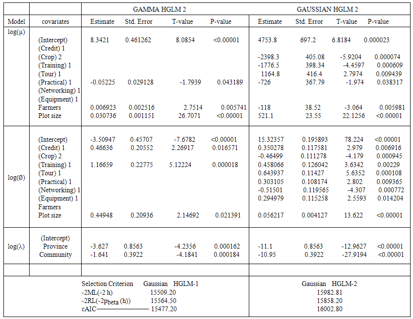 | Table 2. Model Estimates for Gaussian and Gamma distributed HGLM 2 |
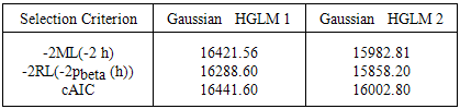
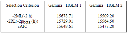
From the dispersion model in table 2, we observe that, in relying on the Gaussian mean model for crop yield, we record a dispersion of 15.323. However we also observe that the contribution of some of the covariates in the dispersion model to this dispersion value increases it while others tend to decrease it. Once a covariate which accounts for the discrepancies can be found, we get a model-based result which can be checked in the future.In the Gaussian model for example, covariates such as access to credit, Training, study tour, demonstrative practical’s, post-harvest equipment’s and plot size increases the dispersion significantly and should be carefully dealt with or checked once we aim at reducing the discrepancies between the data and the fitted values produced by the crop yield model.Also in the Gamma HGLM 2 dispersion model, covariates such as access to credit, Training, and Post-harvest equipment’s tends to increases the dispersion significantly and should be carefully dealt with or checked once we aim at reducing the discrepancies between the data and the fitted values produced by the crop yield model. By model fitness criteria, the Gamma HGLM 2 performed far better than the Gaussian distributed HGLM 2 by both the AIC (−2M L(−2h)), BIC (−2RL(−2pbeta (h)) as well as the cAIC as evident in the last row of table 3.Table 3. Model criteria for Gaussian HGLM 1 and Gaussian HGLM 2
 |
| |
|
3.5. Hierarchical Generalized Linear Models for Quality Improvement
We again seek to strongly recommend that, if we really aim at controlling significantly, the effects of structured dispersions, even in the presence of correlated random errors, the techniques of HGLM 2 as a means of improving the quality should be the number one option. This we have demonstrated using the crop yield data with two random effects resulting from the regional and community variations in this thesis. Table 3 below reveals that the initial Gaussian HGLM even though was satisfactory mixed model (HGLM 1), modelling both mean and dispersion (HGLM 2) improves the quality of the same Gaussian distributed model significantly.Similar can be said of the Gamma HGLM 1 and HGLM 2 as evident in Table 4 below confirming the fact that HGLM 2 improves model quality of mixed models with structured dispersions and significantly reduces the large standard errors resulting from the correlated random effects.Table 4. Model criteria for Gamma HGLM 1 and Gamma HGLM 2
 |
| |
|
4. Discussion
GLMs are extended to generalized linear mixed models (GLMMs), for which the linear predictor of a GLM is allowed to have, in addition to the usual fixed effects, random effects following a normal distribution (Breslow and Clayton, 1993).The Gaussian HGLM 1 diagnostic plots (See Figure 3.5) have some satisfactory features although not the best. The running mean in the plot of residuals against fitted values shows no form of marked trend, even though the plot of absolute residuals has a relatively unstable slope. This does not indicate that the variance is not constant and may not satisfies the independence assumption strictly. It rather suggest the presence of some correlated random effect in the fitted model as expected. The histogram of residuals is almost symmetric. These are satisfactory indications of an appropriate model. Similar is said of the Gamma distributed model in figure 3.6.In both models however (See table 1), plot size cultivated remains the only positive significant contributor to crop yield. High standard errors are observed in the HGLM 1 compared to the GLM and the JGLM and this is due to the presence of correlated random errors resulting from the inclusion of the two random effects; Regions and Communities.
4.1. Hierarchical Generalized Linear Models for Quality Improvement
From figure 3.7 the diagnostic plots have several excellent features compared to the Gaussian HGLM (1) diagnostic plots in figure 3.5. The running mean in the plot of residuals against fitted values displays no form of marked trend at all, and the plot of absolute residuals has an almost stable slope, indicating that the variance is constant and satisfies the independence assumption, that the right link function was specified and also indicates no missing dependency. The normal plot also shows no discrepancy. In addition, the histogram of residuals is almost symmetric. These are very good indications of an appropriate model and an excellent improvement over the counterpart Gaussian HGLM (1) in figure 3.5. The gamma HGLM 2 diagnostic plots of figure 4 also shows an incredible performs over the first gamma HGLM 1 of figure 3.6.Data, fixed unknown constants (parameters) and unobserved random variables (un- observables) are the three objects that form HGLMs. Traditional Bayesian models consist of two objects, data and unobservables, while frequentist’s (or Fisher’s) models consist of the data and parameters. By allowing the three objects in the statistical modeling there is the possibility of describing diverse features in the data, for instance, within-subject correlation in longitudinal studies, smooth spatial and temporal trends, function fittings, and factor analysis, heteroscedasticity, heavy-tailed distributions, robust modellings and sparse variable selections.Table 3 reveals that the initial Gaussian HGLM 1 even though was satisfactory mixed model (HGLM 1), modelling both mean and dispersion (HGLM 2) improves the quality of the same Gaussian distributed model significantly. Similar can be said of the Gamma HGLM 1 and HGLM 2 as evident in Table 4 confirming the fact that HGLM 2 improves model quality of mixed models with structured dispersions and significantly reduces the large standard errors resulting from the correlated random effects.
5. Conclusions
We conclude that, whenever we seek to model fixed and random effects, the HGLM 2 which has the ability of specifying different suitable fixed effects model from a known distribution, a random effects model allowed to follow conjugates of arbitrary distributions from the GLM family and a dispersion model is highly recommended. HGLMs provide valuable class of hierarchical models, giving many inferential tools for testing and checking models, and are particularly helpful for the analysis of data from multi-center field trials. Inferences of both population-average and subject-specific responses can be effectively drawn from a standard HGLM. The GLMM and HGLM 1 are still highly satisfactory statistical models but the HGLM 2 performs far better, gives a more fitting models and improves the quality of the models significantly.
References
| [1] | Breisinger, C., X. Diao, J. Thurlow, B. Yu, and S. Kolavalli. 2008. Accelerating Growth and Structural Transformation: Ghana’s Options for Reaching Middle- Income Country Status. IFPRI Discussion Paper 00750. Washington, DC: IFPRI. |
| [2] | Global Forum on Agriculture 29-30 November 2010, “Economic Importance of Agriculture for Sustainable Development and Poverty Reduction: Findings from a Case Study of Ghana”. Presented to the Working Party on Agricultural Policy and Markets, 15-17 November 2010. Reference: TAD/CA/APM/WP (2010) 40. |
| [3] | Lee Y, Nelder JA. 1996. Hierarchical generalized linear models (with discussion). Journal of the Royal Statistical Society, Series B 1996; 58:619-678. |
| [4] | McCullagh, P. and Nelder, J.A. (1989). Generalized linear models, 2nd ed. Chapman and Hall, London. |
| [5] | Lee, Y. and Nelder, J.A. (1998). Generalized linear models for the analysis of quality-improvement experiments. Canadian journal of Statistics, 26, 95-105. |
| [6] | Lee Y, Nelder J.A., 2001 Hierarchical generalized linear models: a synthesis of generalized linear model, random-effect models and structured dispersions. Biometrika 2001, 88, 4, pp 987-1006. |
| [7] | Youngjo Lee, and J. A. Nelder 2002. "Analysis of ulcer data using hierarchical generalized linear models", Statistics in Medicine, Statist. Med. 2002; 21:191–202 (DOI: 10.1002/sim.978) 01/30/2002. |
| [8] | Jiao H, Wang S, Kamata A. (2005), Modelling local item dependence with the hierarchical generalized linear model. PubMed, J Appl Meas. 2005; 6 (3):311-21. |
| [9] | Jaffrezic F, White IMS, Thompson R, Hill WG. A link function approach to model heterogeneity of residual variances over time in lactation curve analyses. J Dairy Sci. 2000; 83:1089–1093. [PubMed] |
| [10] | Maengseok Noh, Youngjo Lee, Yudi Pawitan, 2005, “Robust ascertainment-adjusted parameter estimation”. Genetic Epidemiology Volume 29, Issue 1, pages 68–75, July 2005. |
| [11] | Noh, M. and Lee, Y. (2006a). Restricted maximum likelihood estimation for binary data in generalised linear mixed models. Journal of Multivariate Analysis, revision. |
| [12] | Noh, M. and Lee, Y. (2006b). Robust modelling for inference from GLM classes. Submitted for publication. |
| [13] | Lars Rönnegård, Majbritt Felleki, Freddy Fikse, Herman A Mulder and Erling Strandberg, 2010. “Genetic heterogeneity of residual variance - estimation of variance components using double hierarchical generalized linear models.” Genetics Selection. |
| [14] | Lars Ronnegard and William Valdar, 2010 “Recent developments in statistical methods for detecting genetic loci affecting phenotypic variability” Genetics Selection Evolution 2010, 13:63http://www.biomedcentral.com/1471-2156/13/63. |
| [15] | Breslow, N.E. and Clayton, D. (1993). Approximate inference in generalized linear mixed models. Journal of the American Statistical Association, 88, 9-25. |
| [16] | Patterson HD, Thompson R. Recovery of inter-block information when block sizes are unequal. Biometrika 1971; 58:545–554. |
 Abstract
 Reference
 Full-Text PDF
 Full-text HTML