1. Introduction

The Fisher hypothesis postulated by Fisher [1] suggests that when expected inflation rises, nominal interest rate will rise with an equal amount without affecting the real interest rate. This implies that a one-for-one relationship exist between the nominal interest rate and the inflation rate. Asemota and Bala [2] noted that this hypothesis has important policy implications for the behavior of interest rates, efficiency of financial markets and the conduct of monetary policy. The Fisher effect is usually tested by imposing rational expectations on inflation forecasts. This is empirically tested by a regression of the nominal interest rate on a constant and the realized inflation. The closer the coefficient of the inflation rate is to one, the stronger the Fisher effect, if the coefficient is substantially different from one, any change in the nominal interest rates will also change the interest rate and may consequently spread to other macroeconomic variables.

Given the important policy implications of the Fisher hypothesis, a large body of research has been devoted to studying the Fisher relation; howbeit, there is no general consensus among researchers on the Fisher hypothesis. Asemota and Bala [2] using the cointegration and Kalman filter approaches could not find evidence of a full Fisher effect for the nominal interest and inflation rates in Nigeria. Also, Engsted [3] and Hatemi-J [4] could not find evidence of the Fisher hypothesis. However, Mishkin [5], Evans and Lewis [6], Wallace and Warner [7], and Crowder and Hoffman [8] found evidence in favour of long-run Fisher effect. Badillo et al. [9] used the panel cointegration approach to analyze the Fisher hypothesis for 15 European Union (EU) countries. The empirical results showed that the coefficient of inflation rate is significantly less than one, which implies the existence of a Partial Fisher effect. Gul and Acikalin [10] using monthly time series could only find evidence of a partial Fisher effect for Turkey.

There are several reasons behind the inability to find evidence of a full Fisher effect. Tobin [11] noted that investors re-balance their portfolios in favour of real assets during high inflationary periods. In addition, the different types of interest rates and sample periods used in the empirical analysis may also affect the results. It may also be due to structural changes in the co-integrating vector. Mishkin [5] noted that the relationship between interest rate and inflation, shift with changes in monetary policy regimes. Chuderewics [12] argued that the Central Bank behavior plays an important role in understanding the varying strengths and weakness associated with the Fisher relation. He developed a theoretical model that incorporates Central Bank behavior and demonstrated that the strength of the Fisher relation depends explicitly on its behavior. Recently, more attention has been given to investigations of possible structural breaks in macroeconomic time series. Hatemi-J [4] argued that the inability to find a full Fisher effect may be due to parameter instability. Structural breaks may occur due to financial crises, policy changes, changes in consumers’ preferences and behavior, technological changes and political instability, among others.

The aim of this paper is to empirically investigate the Fisher effect in selected ECOWAS¹ countries by employing annual data from 1961 to 2011. The inflation and interest rates for Burkina Faso, Cȏte d’Ivoire, Gambia, Ghana, Niger, Nigeria, Senegal and Togo are used in the study. First, we investigate the order of integration of the 16 time series using the augmented Dickey-Fuller (ADF), Phillips-Perron (PP) and the Kwiatkowski-Phillips- Schmidt-Shin (KPSS) unit root tests. We apply different lag selection criteria for the ADF tests and different methods are used for the computation of the long-run variance for PP and KPSS tests. These were conducted to ascertain if inferences based on unit root tests are affected by the method of lag selection and method of constructing heteroskedasticity and autocorrelation consistent (HAC) estimators. In addition, we also conducted unit root tests allowing for one and two endogenous structural breaks. To examine the dynamic relationship between inflation and nominal interest rate, the time varying parameter model is constructed and the Kalman filter estimation method is utilized to estimate and show the varying strength of the response of the interest rates to changes in inflation. Finally, the Harvey-Koopman technique is employed to detect the time of structural breaks and outliers in the constructed models. This is the first attempt in the literature to examine the Fisher effect using Kalman filter methodology in the ECOWAS region and it is aimed at filling an important gap in the empirical literature on developing countries. In addition, the paper is one of the few studies that empirically compare and provide evidence on the performance of the PP and KPSS test when different methods are used in the computation of the long-run variance. The rest of the paper is organized as follows: section 2 describes the methodology. Section 3 presents the data and the empirical findings, and the last section concludes.

2. Econometric Methodology

2.1. Unit Root Tests without Structural Breaks

It is now a tradition in the field of econometrics to investigate the order of integration of macroeconomic variables prior to modeling the series. This is necessary in order to avoid the problem of spurious regression as first pointed out by Granger and Newbold [13]. Mishkin [5] argued that both inflation and interest rates contain unit roots, hence, the “traditional” forecasting equation suffers from the spurious regression problem, except, if the variables are cointegrated. The augmented Dickey-Fuller (ADF), the Philips-Perron (PP) and the Kwiatkowski– Phillips–Schmidt–Shin (KPSS) tests will be used in this study to examine the order of integration of the 16 macroeconomic variables. The augmented Dickey–Fuller (ADF) test (Dickey and Fuller 1979 [14]) is based on the following model:

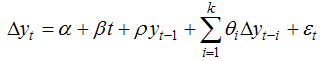(1)

where is a well behaved error tem²; is the lagged first difference added to correct for serial correlation in the error and the maximum lag is selected using the Schwartz information criterion (SIC) and the ‘t sig’ approach proposed by Hall [15] and , , and are the parameters to be estimated. Equation (1) tests the null hypothesis of a unit root against a trend stationary alternative.

The Philips–Perron [16] method estimates the test equation below:

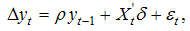(2)

The PP test is based on the statistic which modifies the Dickey–Fuller test. Where is the estimate, the t–ratio, is coefficient standard error, and is the standard error of the test regression. Further, is a consistent estimate of the error variance in (2), while is an estimator of the residual spectrum at frequency zero. The lag window or bandwidth use in the study is estimated by two criteria; the Newey-West criterion (Newey and West, [17]) using the Bartlett kernel and the Andrews criterion (Andrews [18]) using the quadratic spectral kernel.

However, Kwiatkowski et al. [19] argued that the classical method of hypothesis testing is biased towards the null hypothesis. Hence, it ensures that the null hypothesis is accepted unless there is strong evidence against it. They pointed out that the standard unit root tests are not very powerful against relevant alternatives; see (Kwiatkowski et al. [19], pg. 160). To circumvent this problem, KPSS [19] proposed a test of the null hypothesis that a series is stationary around a deterministic trend. They concluded that by testing both the unit root null hypothesis and the stationarity null hypothesis, researchers can distinguish series that appear to be stationary, those that appear to have a unit root, and those that the data (or the tests) are not sufficiently informative to decide whether they are stationary or integrated. The KPSS test is given by the following equations:

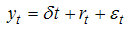(3)

where is a stationary error and is a random walk given by:

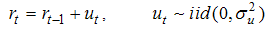(4)

The initial value is treated as fixed and serves as the intercept in the model and the null hypothesis of stationarity is formulated as or is constant. The LM statistic is given by:

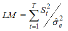(5)

where are residuals from the regression of on an intercept and time trend, is the estimate of the error variance of the regression and is the partial sum of defined by:

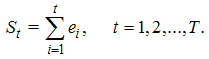(6)

When the errors are the estimator converges to , however, when the errors are not , a consistent estimator of the long-run variance is given by:

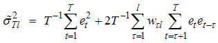(7)

where is an optimal weighting function that corresponds to the choice of a spectral window. KPSS use the Bartlett window suggested by Newey and West [17]. The modification is given by:

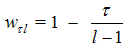(8)

However, Leybourne and McCabe [20] argued that inference from the KPSS test can be very sensitive to the value of the lag that is used in the computation of the . Hence, in this paper, we also consider Andrews’ [18] quadratic spectral kernel in the computation of the long-run variance to ascertain the degree of sensitivity of the KPSS test to the different method of computation of heteroskedasticity and autocorrelation consistent long-run variance.

2.2. Unit Root Tests with Structural Break

2.2.1. Zivot-Andrews Unit Root with one Structural Break Test

Starting with the pioneer work of Perron [21], it has been proved that conventional unit root tests are biased towards the non-rejection of the unit root null hypothesis even if the data are stationary with structural break(s). Perron [21] incorporated dummy variables in the ADF test to account for one exogenous structural break. However, this exogenous imposition of break date has been criticized by Christiano [22] and Zivot-Andrews [23]. Zivot-Andrews [23] proposed a data dependent algorithm to determine the breakpoint. The Zivot-Andrews test is carried out using the following regression equations:

Model A (Crash Model):

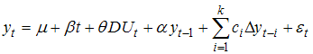(9)

Model B (Changing Growth Model):

(10)

Model C (Mixed Model):

(11)

where if 0 otherwise; if 0 otherwise, is the date of the endogenously determined break. Model A, referred to as the “crash model” allows for a one-time change in the intercept of the trend function, model B, referred to as the “changing growth model” allows for a single change in the slope of the trend function without any change in the level; and model C, the “mixed model” allows for both effects to take place simultaneously, i.e., a sudden change in the level followed by a different growth path. ³ The null hypothesis for the three models is that the series is integrated (unit root) without structural breaks (α = 1). The test statistic is the minimum “ ” over all possible break dates in the sample. Zivot-Andrews [23] suggested using a trimming region of (0.10T, 0.90T) to eliminate endpoints.

2.2.2. Lagrange Multiplier (LM) unit Root Test with Structural Breaks

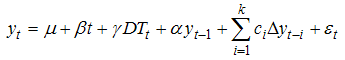
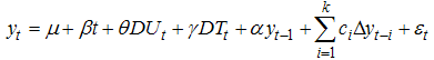
Lee and Strazicich [25] argued that the Zivot-Andrews test omit the possibility of unit root with break. Hence, researchers may incorrectly conclude that a time series is stationary with breaks when in fact the series is nonstationary with break(s). To circumvent this problem, they proposed the minimum LM unit root test in which the alternative hypothesis unambiguously implies trend stationarity. The LM unit root test can be explained using the following data-generating process (DGP):

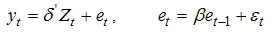(12)

where is the observed time series, is a vector of coefficients, is a vector of exogenous variables and is a well-behaved error term. Corresponding to the two-break equivalent of Perron’s [21] Model C, with two changes in the level and the trend, is defined by 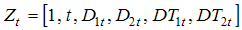to allow for a constant term, linear time trend, and two structural breaks in level and trend.⁴ Under the alternative hypothesis, the terms describe an intercept shift in the deterministic trend, where = 1 for , = 1, 2, and 0 otherwise; denotes the time period when a break occurs and describes a change in slope of the deterministic trend, where 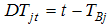for 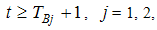and 0 otherwise. 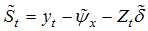Note that the DGP includes breaks under the null and alternative hypothesis in a consistent manner.

Lee and Strazicich [25] used the following regression to obtain the LM unit root test statistic:

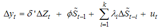(13)

where , = 2, … , is a de-trended series; are coefficients in the regression of on ; is given by ; and denote the first observations of and respectively. Vougas [27] has shown that the LM type test using the above optimal de-trending device is more powerful and finds more evidence in favor of trend stationary than the ADF type test. , = 1, …, terms are included as necessary to correct for serial correction. Note that the test regression (12) involves instead of so that becomes 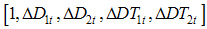. The unit root null hypothesis is described by , and the LM test statistics are given by:

(13a)

(13b)

To endogenously determine the break points , the minimum LM unit root test uses a grid search as follows:

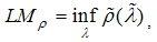(14a)

(14b)

Where , and is the sample size. Vougas [27] indicated that in the application of LM test, the studentized version takes into account the variability of the estimated coefficients and is more powerful than the coefficient test . The breakpoints are determined to be where the test statistic is minimized. As is typical in endogenous break test, we use a trimming region of (0.15T, 0.85T) to eliminate endpoints. Critical values are tabulated in Lee and Strazicich [25].

2.3. The State Space Model

The Fisher effect is usually investigated by regressing the nominal interest rate on a constant and the realized inflation rate. The value of the coefficient on the inflation rate provides a measure of the Fisher effect. The closer the value of the coefficient is to one, the stronger the Fisher effect. The Fisher effect is usually represented by the following equation:

(15)

where is the nominal interest rate, is the ex-ante real rate of interest and is the expected inflation rate. Assuming rational expectations on the inflation forecasts implies that;

(16)

where the forecast error is white noise. Hence, the regression equation for Fisher effect is:

(17)

The strength of the Fisher effect is usually assessed by comparing the coefficient of inflation to one. If in equation (17), we have the full Fisher effect, however, if it is known as the partial Fisher effect. The specification in (17) above assumes that the coefficient is constant throughout the time under investigation. This specification may be spurious especially in economic and business applications where the level of randomness is high, and also where the constancy of patterns or parameters cannot be guaranteed. In addition, the monetary policy behavior of the central banks is not constant through time. Thus, to capture the dynamic economic environment and the evolving policy behavior, a more flexible model that allows the parameter to vary randomly over time is adopted. This flexible model is popularly referred to as the time varying parameter model. The state space representation of (17) as a time varying parameter model is given as:

(18)

The first equation in (18) is called the measurement equation while the second is the state or transition equation. The measurement equation relates the observed variables (data) and the unobserved state variable (), while the transition equation describes the evolution of the state variable. The observation error and state error are assumed to be Gaussian white noise (GWN) sequences. The overall objective of state space analysis is to study the evolution of the state () over time using observed data. When a model is cast in a state space form, the Kalman filter is applied to make statistical inference about the model. The Kalman filter (hereafter, KF) is simply a recursive statistical algorithm for carrying out computations in a state space model. A more accurate estimate of the state vector or slope coefficient can be obtained via Kalman Smoothing (K.S). The unknown variance parameters ( and ) in model 12 are estimated by the maximum likelihood estimation via the Kalman filter prediction error decomposition initialized with the exact initial Kalman filter. Harvey and Koopman [28] demonstrated that the auxiliary residuals in the state space model can be very informative in detecting outliers and structural change in the model. For a complete exposition of the state space model and Kalman filter, see Durbin and Koopman [29] and Hamilton [30].

3. Data, Results and Discussion

3.1. The Data

The data used in this study are obtained from the International Financial Statistics (IFS) database CD-ROM (June, 2012). We utilize annual inflation and nominal interest rates data of ECOWAS countries over the time period of 1961-2011 depending on data availability.⁵ A time series plot of the series for the different countries is depicted in figure 1.

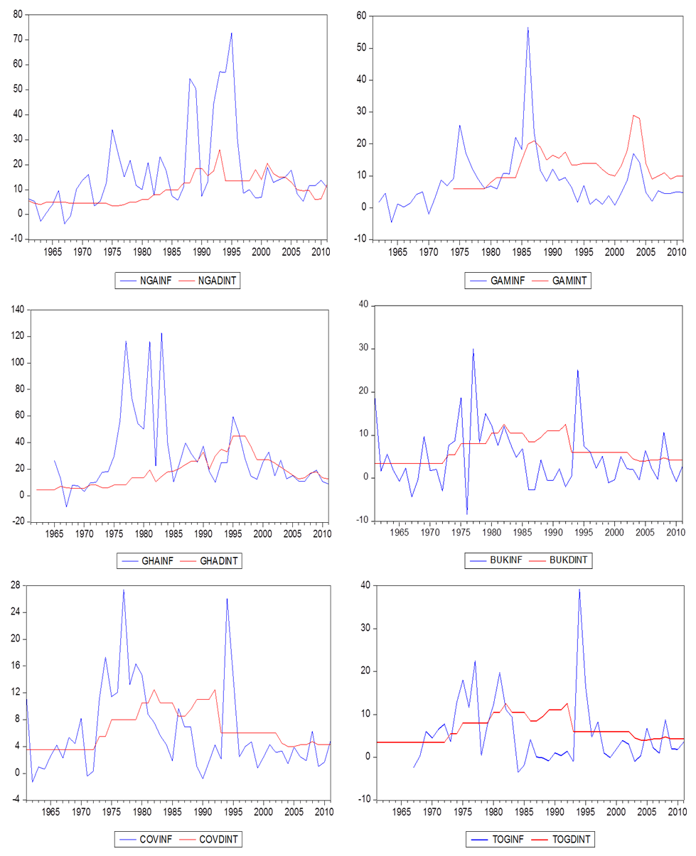Figure 1. Time Series Plots of Inflation and Interest Rates for the ECOWAS countries

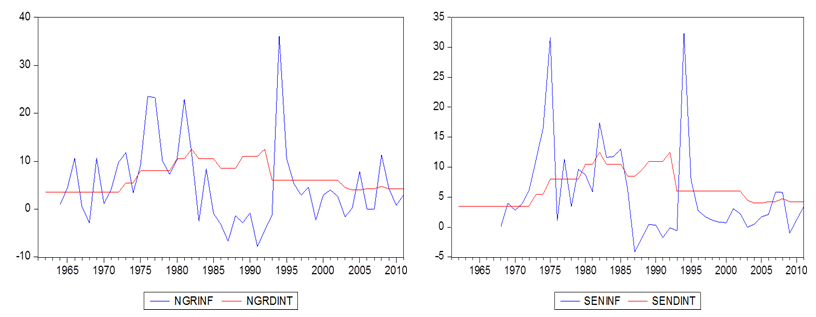Figure 1. Continued

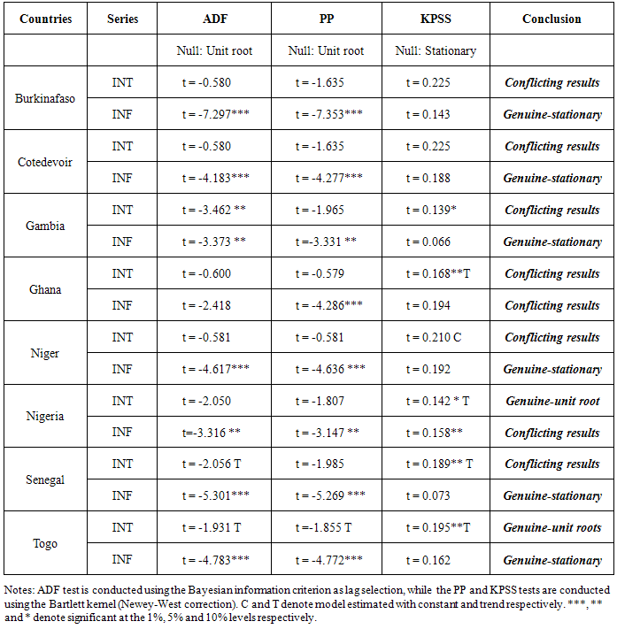
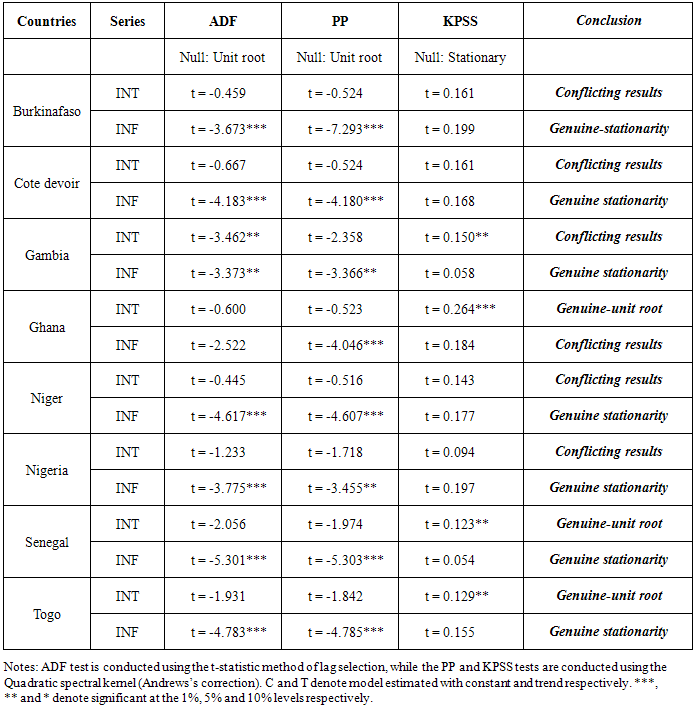
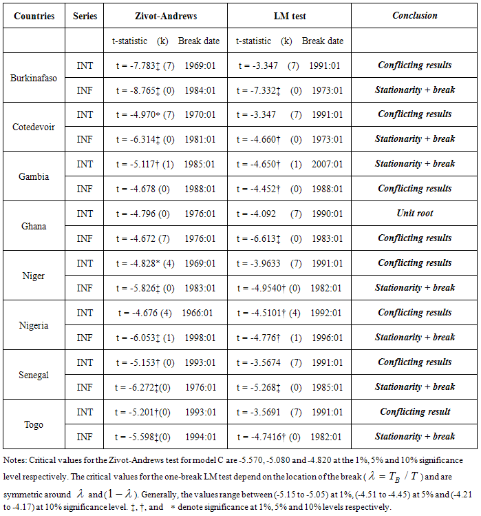
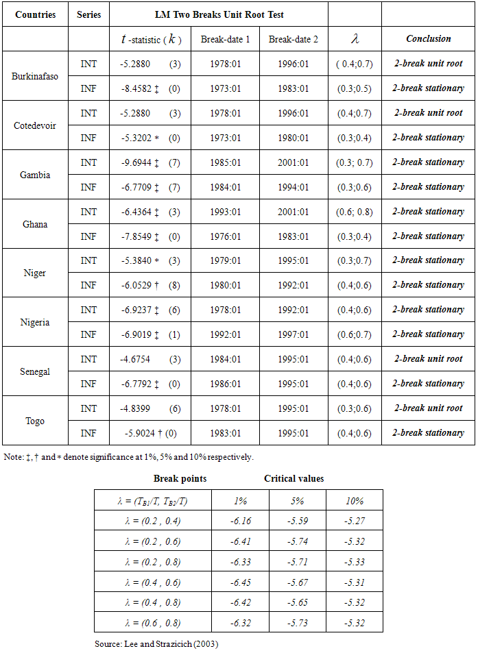
3.2. Unit Root with and without Structural Breaks Tests Results

It has now become standard practice in time series analysis to investigate the order of integration of the series prior to its statistical modeling. In the econometric literature, the augmented Dickey-Fuller test is most commonly used to ascertain the order of integration of the time series data. In addition, we also apply the Phillips-Perron [16] and the Kwaitkowski et al. [19] tests to the series while varying the method of lag selection (for the ADF test) and the method of correction for autocorrelation and heteroskedasticity (PP and KPSS tests).

The conventional unit root tests (ADF, PP and KPSS) that do not allow for the possibility of structural breaks have been proven to be biased towards the non-rejection of the null hypothesis. Hence, we also apply the one-break and two-break unit root tests. The results are provided in the table 1.

Table 1. Unit root tests without structural breaks

The results of the various unit root tests displayed in Table 1 reveal some interesting findings. The ADF test that utilizes the Schwarz information criterion rejects the unit root null for 8 of the 16 series, while the Phillips-Perron test that utilizes the Bartlett kernel in the computation of the long-run variance also rejects the unit root null for 8 of the 16 series. With the KPSS test, we cannot reject the null of stationarity at the usual critical levels for 10 series when the Bartlett kernel is used as the method for heteroskedasticity and autocorrelation correction. The overall conclusions of the confirmatory analysis are quite contradictory: the confirmatory analysis yield 8 cases of conflicting results; a situation where the individual test arrives at different conclusion, 6 cases of genuine-stationarity and 2 cases of genuine-unit root process. We then alter the method of lag selection for the ADF test to the t -statistic approach and the method of computation of the long-run variance to the quadratic spectral kernel for the Phillips-Perron and KPSS tests. The results in Table 2 reveals that the ADF and the Phillips-Perron tests also rejected the unit root hypothesis for 8 of the 16 series, while the KPSS test cannot rejects the null hypothesis of stationarity for 12 of the 16 series.

Table 2. Unit root without structural breaks

The overall confirmatory analysis using the three tests indicated conflicting conclusions for 6 series, 7 series with genuine-stationarity and 3 series with genuine-unit root conclusion. Based on these findings, we can say that the ADF and the Phillips-Perron test displays a considerable degree of robustness to the method adopted in correction for heteroskedasticity and autocorrelation while the robustness of the KPSS test to the method of computation of the long-run variance is weak.

We also conducted unit root test that account for the possibility of one and two endogenous breaks in the specification. The Zivot-Andrews and the minimum Lagrange multiplier endogenous break results are reported in Table 3 while the results of two-breaks are reported in Table 4.

Table 3. Unit root with one structural break

Table 4. Two-break unit root test

At the conventional significance level, the ZA test rejects the unit root null for 12 of the 16 series; this implies that, 12 series are found to be stationary with one structural break. The minimum LM test rejects the null hypothesis of unit root with one break for 10 of the 16 series; therefore, we find evidence of stationarity with one structural break for 10 series. The combined analysis of both results yield 8 conflicting conclusions, 7 cases of genuine cases of stationarity with one structural break and 1 case of genuine unit root. The different break dates selected by the ZA and minimum LM one-break test and the 50% conflicting conclusion in the combined analysis of both tests are puzzling.

Ohara [31] noted that just as the unit root tests that fail to account for structural breaks are biased towards the non-rejection of the null hypothesis, under specification of the number of break may also lead to misleading inferences. Hence, we also report the results of the minimum Lagrange multiplier two-break unit root tests in table 4. Using the two-break LM test, we find evidence of stationarity with two-break points for 12 of the series. Kwiatkowski et al. [19] noted that the test of the unit root null hypothesis should be complemented by the test of the null hypothesis of stationarity for confirmatory analysis, i.e., to ascertain our conclusion about the unit roots. However, this assertion has been regarded as an illusion by Burke [32] who through a detailed Monte Carlo study reveals that the KPSS test has the same poor power properties as the ADF test. He concluded that even if confirmation occurs, it may be incorrect. In addition, the different break dates in our results and the issue of the actual number of breaks to be included in the unit root test with structural breaks still remains controversial in the literature. For example, the one-break endogenous test results of Zivot-Andrews yields 12 stationarity with breaks series, while the minimum LM test yields 10 stationarity with break series. Which is the more powerful of the two tests? Furthermore, applying the two-break LM test also yields 12 stationary series with two structural breaks. What if there are more than two structural breaks? Hence, in the face of all these issues, why testing for unit root in macroeconomic time series then? According to Harvey [33], “why worry about testing for unit roots in the first place’’? A more recent direction in econometrics is the modeling of macroeconomic series in the framework of state space models. In the state space framework, structural change is accounted for in the model building methodology and testing for non stationarity is not important. Hence, in the next section, we assess the strength of the Fisher relationship using the time varying parameter model estimated by the Kalman filter methods.

3.3. The State Space Model Estimation Results

We employed the time varying parameter techniques to capture the behavior of interest rates to changes in the inflation rates over time. The relationship is examined in the state space framework and the Kalman algorithm is apply to assess if this relationship is stable through time. Prior to Kalman filtering and smoothing, we estimate the unknown variance parameter of the model using the maximum likelihood method maximized by the BFGS (Broyden-Fletcher-Goldfarb-Shannon) method. After estimating the unknown variances, the Kalman filter technique is applied to estimate the time path of the parameter of interest (Fisher coefficient). The Kalman filter estimate of the behavior of the parameter is depicted in figure 2.

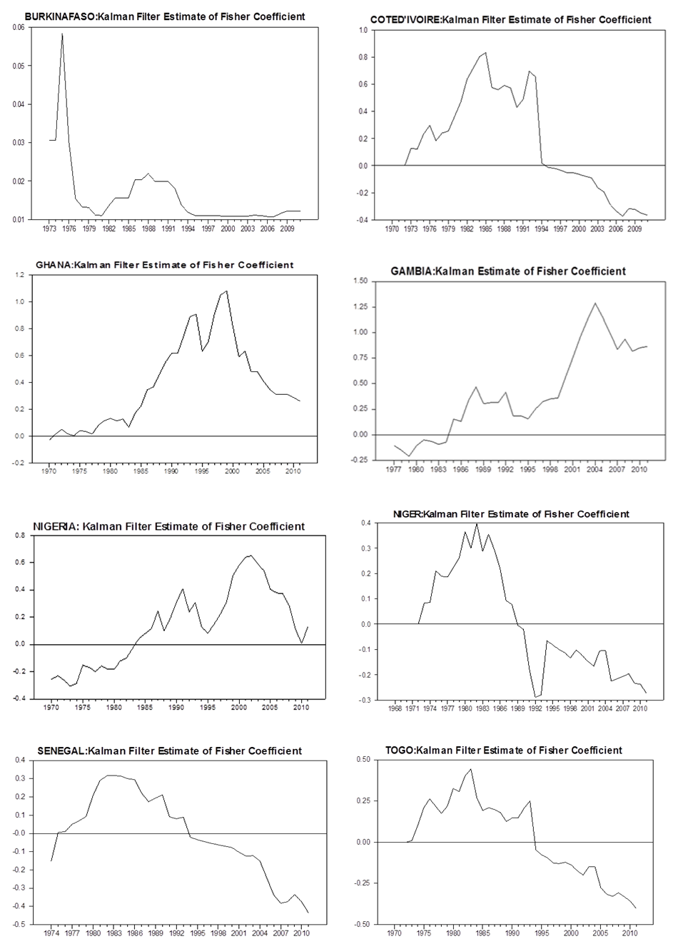Figure 2. Kalman Filter Estimate of the Fisher Coefficient for the ECOWAS Countries

The plots in Figure 2 indicate that the relationship between interest and inflation rates vary over time and the variation in the strength of the Fisher effect varies among countries. The plots indicate that the strength of the Fisher effect fluctuates around 0.01 to 0.06 for Burkina Faso during the period from 1973 to 2011, while for Ghana, the strength of the Fisher effect hovers around 0.2 to 1.1 during the period from 1980 to 2011. In fact, in the case of Ghana, we can say a full Fisher effect exists between the periods from 1997 to 2000. However, this full Fisher effect gradually decline to partial Fisher effect from 2001 until the end of the sample. In the case of Gambia, the strength of the Fisher effect was 0.20 to 1.25 during the period from 1985 to 2011. The strength of the Fisher relationship gradually increased from the mid-1990s and attained a full Fisher effect in the early 2000s and relatively maintained the high strength through the sample period. The strength of the Fisher relationship for Nigeria was around 0.20 in the mid-1980s and attained its highest strength of 0.60 in the early 2000s and gradually declines afterwards. There is no noticeable period of full Fisher effect in the case of Nigeria over the period under consideration. With the exception of Cote d’ivoire that attained a relatively full Fisher effect in the mid-1980s, for all the other Francophone ECOWAS countries, there is no noticeable period of full Fisher effect over the period of study. For example, the strength of the Fisher relationship increased from 0.1 in 1980 to about 0.3 in 1985 and gradually decreased afterwards until it drifted into the negative axis from 1994. Hence, a partial Fisher effect exists for Senegal around 1974 to 1993. Similarly, in the case of Togo, the strength of the relationship increased from the early 1970s to about 0.4 in 1983 and gradually decreased afterwards until it drifted into the negative axis in 1994. An interesting result about the Francophone ECOWAS countries, is the sudden drift of the Fisher effect parameter into negative territory in 1994 (with the exception of Niger). Hence, a pondering question is; why did the parameter of the Fisher effect drifts into the negative axis for the Francophone ECOWAS countries in 1994? This may be as a result of sharp and strong devaluation of the CFA franc (a common currency for the ECOWAS francophone) that occurred in January 1994. Prior to devaluation, the value of CFA has been criticized as being too high, and only favors the urban elites of the ECOWAS francophone countries at the expense of the farmers who cannot easily export their agricultural products. Hence, the devaluation of the 1994 was aimed at addressing these imbalances.

Our results indicate that the strength of the Fisher effect does vary over time. Specifically, for the ECOWAS countries; in some periods there appears to be a strong relationship between the interest and inflation rates (full Fisher effect), while in other periods, the relationship seems to be weak (partial Fisher effect) and non-existing at some other periods. The variation in the strength of the Fisher effect may be attributed to the monetary policies adopted by the central banks at different time periods. Chuderewicz [12] has demonstrated using a theoretical model that the strength of the Fisher relation depends explicitly on the behavior of the central bank. He noted that the higher the degree of commitment of central banks to monetary targets, the stronger is the relationship between the interest and inflation rates. Hence, we recommend that monetary authorities in the ECOWAS countries should aim at making more effective monetary policies and demonstrate strong commitments to monetary targets in order to strengthen the Fisher relations.

3.4. Structural Breaks and Outliers Detection Results

We exploit the capability of the state space model in detecting the time of structural breaks and outliers. Harvey and Koopman [28] demonstrated that auxiliary residuals in state space models are potentially useful not only for detecting outliers and structural breaks but for distinguishing between them. The auxiliary residuals are estimators of the disturbances associated with the unobserved components. The detection strategy is to plot the standardized residuals. In a Gaussian model, indicators of outliers and structural breaks arise for values greater than 2 in absolute value. We apply this procedure to the standardized observation equation residuals and the state equation residuals in (18) to detect outliers and time of structural breaks respectively. The plots are presented in Figure 3.

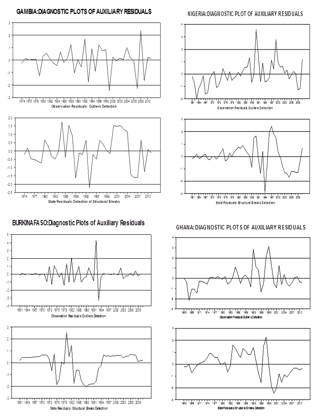Figure 3. Detecting Outliers and Structural Breaks

The plots of the auxiliary residuals for Burkina Faso, Gambia, Ghana and Nigeria (others are available on request) are shown in figure 3. Outliers are detected in the Fisher relations in 1992 and 1993 for Burkina Faso, in 1994 and 1996 for Gambia, 1992 and 1998 for Ghana and 1990 and 1999 for Nigeria. The plots of the other countries also reveals the presence of outliers in the Fisher relation for Togo in 1992, 1989, 1990 and 1992 for Cote d’ivoire, 1992 for Niger, and 1991 and 1992 for Senegal.

On the basis of the plots, we find evidence of structural breaks in the Fisher relationship in 1980 for Burkina Faso, 1980, 1981, 1993-1994 for Cote d’ivoire, around 2005-2007 for Gambia and 1997 and 1999-2000 for Ghana. We also detect structural breaks in 1994, 1997-1998 for Nigeria, 1985-1986 for Niger, 1972-1974 for Senegal and 1973-1975 for Togo.

4. Conclusions

This paper empirically investigates a fundamental relationship in macroeconomics: the relationship between interest and inflation rates. The fundamental issue addressed in this paper is whether this relationship is stable over time for ECOWAS countries. The inflation and interest rates for Burkina Faso, Cȏte d’Ivoire, Gambia, Ghana, Niger, Nigeria, Senegal and Togo are used in the study. First, we investigate the order of integration of the 16 time series using the augmented Dickey-Fuller (ADF), Phillips-Perron (PP) and the Kwiatkowski-Phillips-Schmidt-Shin (KPSS) unit root tests as a confirmatory test. Using the BIC as the lag selection criteria for the ADF test and the Bartlett kernel for the computation of the covariance matrix for both the PP and KPSS, the results yield 8 cases of conflicting results, 6 cases of genuine-stationarity and 2 cases of genuine-unit roots. When the -statistic is used for the selection of the lag order for the ADF test and the Quadratic Spectral kernel is used for the PP and KPSS, the test results indicate 6 cases of conflicting results, 7 cases of genuine-stationarity and 3 cases of genuine-unit roots. This indicates that inference based on unit root tests may be affected by the method of lag selection and method of constructing heteroskedasticity and autocorrelation consistent (HAC) estimators. We also conduct unit root tests allowing for one and two structural breaks. On allowing for structural breaks, the unit root hypothesis is rejected for 12 out of the 16 series considered in the study. Secondly, the Fisher equation is cast in the state space form and the Kalman filter is apply to estimate the slope parameter. Our results indicate that the strength of the Fisher effect does vary over time. Specifically, for the ECOWAS countries; in some periods there appears to be a strong relationship between the interest and inflation rates (full Fisher effect), while in other periods, the relationship seems to be weak (partial Fisher effect) and non-existing at some other periods. Using the Harvey-Koopman procedure, we detect the time of structural breaks and outliers in our model. Finally, we recommend that monetary authorities in the ECOWAS countries should aimed at making effective monetary policies and demonstrate strong commitments to monetary targets in order to strengthen the Fisher relation.

ACKNOWLEDGEMENTS

We thank Professor Peter C. B. Phillips, Felix Chan and other participants at the New Zealand Econometric Study Group Meeting 2013 for their helpful comments when this paper was first presented at the New Zealand Econometric Society Conference. The usual disclaimer applies.

Notes

1. ECOWAS is an acronym for Economic Community of West African States. It is a regional group of fifteen countries founded in May 28, 1975 to promote cooperation and integration, with a view to establishing an economic and monetary union as a means of stimulating economic growth and development in West Africa.

2. The error term is said to be well–behaved if it is independently and identically normally distributed.

3. Perron [21] suggest that most macroeconomic time series can be adequately modeled using either model A or model C. In addition, Sen [24] argued that if one assumes that the location of the break is unknown, it is most likely that the form of the break will be unknown as well. Sen [24] demonstrated that the loss in power is quite negligible if the mixed model specification is used when in fact that the break occurs according to the crash model or changing growth model, and concluded that practitioners should specify the mixed model in empirical applications. Hence, we used model C in our empirical analysis.

4. Lee et al. [26] noted that there are technical difficulties in obtaining relevant asymptotic distributions and the corresponding critical values of endogenous test with three or more breaks.

5. The inflation and interest rates for Burkina Faso, Cȏte d’Ivoire, Gambia, Ghana, Niger, Nigeria, Senegal and Togo are used in the study. The other ECOWAS countries are omitted from the study because the data available on their inflation and interest rates are too scanty to be included in the analysis.