1. Introduction

Sample data collected for regions or points in space are not independent, but rather spatially dependent, which means that observations from one location tend to exhibit values similar to those from nearby locations. For many social and economic processes, a better appreciation of the spatial context can potentially avoid misleading inferences and improve the strength of results and their interpretation. Knowledge about the location of a process and its interaction with processes at neighboring locations can help infer the underlying reasons and logic of the process under investigation.

Existing regression models used to analyze cross-section and panel data assume that observations/regions are independent of one another. However, in real life this is not usually the case. For instance, a conventional regression model that relates commuting times to work for region i to the number of persons in region i utilizing different commuting modes and the density of commuters in region i, assumes that mode choice and density of a neighboring region, say j does not have an influence on commuting time for region i. Since it seems unlikely that region i’s network of vehicle and public transport infrastructure is independent from that of region j, we would expect this assumption to be unrealistic. Ignoring this violation of independence between observations will produce estimates that are biased and inconsistent. In addition, misspecification increases the probability of wrong inferences at least as much as does the choice of a biased or inefficient estimator.

Analysis of economic data explicitly linked to location can be approached from two spatial econometrics perspectives namely, spatial heterogeneity and spatial autocorrelation. Spatial heterogeneity might arise due to a lack of structural stability across space, such as varying parameters or functional forms, and due to non homogeneity of the units of observations across space. While, spatial autocorrelation refers to the lack of independence among observations: similar to autocorrelation in time-series models (Anselin 1988).

Spatial autocorrelation among observations and the importance of relative locations is expressed in Tobler’s first law of geography, which states that “everything is related to everything else, but near things are more related than distant things”. Interactions among neighboring agents could, for example, induce a correlation of the variables across space, which must be accounted for in model estimation Tobler (1979).

Theoretical motivations for the observed dependence between nearby observations are countless. For instance, Ertur and Koch (2007) used a theoretical model that posits physical and human capital externalities as well as technological interdependence between regions. The study showed that this leads to a reduced form growth regression and that an average of growth rates from neighboring regions should be included.

Thomas Plümper and Eric Neumayerb (2010) identified four specification issues in the analysis of spatial data. They argued that to avoid biased estimates of the spatial effects, researchers need to consider carefully how to model temporal dynamics, common trends and common shocks, as well as how to account for spatial clustering and unobserved spatial heterogeneity. Failure to model temporal dynamics and to control for common shocks and common trends in cross-sectional, time-series or panel data is likely to bias the estimated coefficient of the spatial effect variable, with the bias often being upward. In addition, failure to model appropriately spatial patterns in the dependent variable could lead to bias in the spatial effect estimation.

This study investigates the significance of incorporating spatial effect into regression analysis. The purpose is to build a spatial and non spatial model, design a Monte-Carlo experiment and observe the point of convergence in the two models. The specific objective is to observe the bias that could emanate from omitting spatial effect in SAR model when it exists and to examine the relationship of the bias with degree of spatial autocorrelation.

The present study is a contribution to existing work on incorporating locational aspect of sample data into the model. It is different from the existing work in that its discriminate between spatial and non spatial models, observe point of convergence in the two models, investigate bias emanating from omitting spatial effect when its exists. Also, it provides information on association between this bias and degree of spatial autocorrelation through a well-designed Monte Carlo experiment.

The rest of the paper is organised as follows: review of literature, model specification and estimation techniques, Monte Carlo design, result presentation and discussion, and concluding remark.

2. SAR Model Specification and Estimation

Spatial autoregressive (SAR) model with lagged dependent variable is given as:

(1)

Where:

vector of regression coefficients

vector of explicative variables at site

vector of lagged dependent variable

= the elements of a row-standardized weight matrix

= Spatial effect coefficient and error term

Unlike the case of the time series analogous specification, the presence of the spatial lagged term amongst the explicative variables induces a correlation between the error and the lagged variable itself (see Anselin and Bera, 1998). Put differently, we would not want to run OLS on this model, since the presence of on both the left and right sides means that we have a correlation between errors and the regressors and the resulting estimates will be biased and inconsistent.

Equation 1 can be written in a more compact matrix notation as

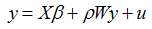(2)

Where:

vector of independent and identically distributed (iid) disturbances

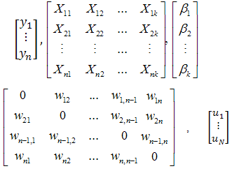The reduced form of equation 1 is obtained as follows

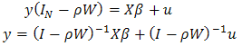(3)

(4)

Under the hypothesis of normality of the error term, the log-likelihood function of the model 1 is given by:

(5)

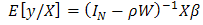
Analytical solution for , conditional on and given respectively as:

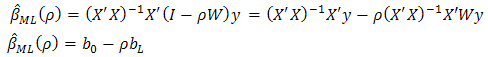(6)

Where

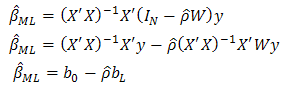
Inspection show that is the coefficient vector from the OLS regression of , while is from OLS regression of . So if is known, we could compute the ML estimate of . As a consequence, the residuals of these two OLS regressions are given as:

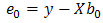(7)

(8)

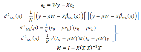
Expression in 8 can be substituted into 5 to write a version of the log-likelihood function in terms of only. This yields the concentrated log-likelihood which is given as:

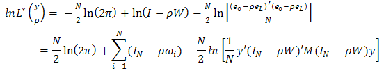(9)

Maximizing this is equivalent to minimizing

(10)

This is also equivalent to

(11)

There is need to impose a constraint on the parameter . Anselin and Florax (1994) point out that the parameter can take on feasible values in the range . This requires that we constrain our optimization search to values within this range. Note that are respectively minimum and maximum Eigen value of W.

The estimator is then substituted into the solution for to yield :

(12)

The steps involved in the ML estimation of the model are summarized below as:

i. Perform OLS for the models

ii. Compute residuals

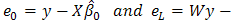
iii. Given , find that maximizes the concentrated likelihood function obtained in 9

iv. Given that maximizes the concentrated ML, compute 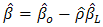and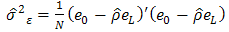

(13)

3. Monte Carlo Analysis

In this section, in an attempt to assess the performance of the OLS estimator when spatial autocorrelation is ignored series of Monte Carlo experiments were set up. When spatial autocorrelation consistent with a diffusion process exists in the data generating process and a spatially lagged dependent variable is omitted from the model, OLS parameter estimates for the remaining covariates will be biased and inconsistent. In the Monte Carlos, the Data Generating Process (DGP) for the case of spatial autocorrelation takes the form:

(14)

Where . The independent variable, , is normally distributed with a mean of 0 and a standard deviation of 3. Also, β₀ and β₁ are set to one (1).

The study examines the bias of the OLS estimates of β1 when spatial autocorrelation in the DGP are omitted from the OLS specification. In addition, the study investigate the performance of OLS varying both the number of observations (and the corresponding spatial weights matrices) and the degree of spatial autocorrelation, as reflected in the autoregressive parameters .

For each set of experiments, the observations are arrayed in regular square lattices. Monte Carlos is performed for four different sizes of square lattice structures: a . In each case a queen contiguity definition of neighbours is employed. The performance of OLS is examined for five values of For each combination of lattice size and , 1000 replications were performed.

In order to implement the estimation techniques discussed in the previous section and to observe the distribution of in the simulation, R statistical software code was developed.

4. Monte Carlo Result

This section of the study presents the result of the Monte Carlo design discussed earlier. To allow for simplicity, the section is divided into two. The first focus on the comparison of OLS and SAR model and contain information on the point of convergence of the two models. The second subdivision furnishes information on the relationship between biases of omitting spatial in SAR and the degree of spatial autocorrelation. These are discussed sequentially below.

4.1. OLS versus SAR Model

Table 1 shows the result for OLS and SAR model respectively for various numbers of observations considered in the simulation. From the table, (especially when N= 25 and 100) the consequences of taking spatial effect into account are quite clear. The residual standard error of spatial models is much smaller than that of the least squares regression counterpart. In essence, spatial model performs better than the OLS especially where spatial effect parameter is highly significant as indicated by LM, LR and Wald diagnostic test result for spatial dependence.

Table 1. OLS versus SAR model

From table 1, the result of the three approaches considered to examine the presence of spatial effect in the data set was found to have the same results. For N=25 and 100 spatial effect parameter is found to be significant and for N= 400 and 900 the null hypothesis of absence of spatial effect are accepted. The results obtained in these two cases are not significantly different from OLS result. Hence, it is of no use to go for the spatial model when it has been confirmed by a diagnostic test-statistic that spatial effect does not exist in the dataset.

4.2. Relationship between Bias of Omitting Spatial Effect and Degree of Spatial Autocorrelation

This segment of the paper examines the relationship between bias of omitting spatial effect and the degree of spatial autocorrelation. In the simulation, the values of spatial effect parameter are fixed, varying the number of observation and the corresponding lattice size replicated 1000 times. In each case, the density of is shown so as to clearly know how the bias emanating from omitted spatial is related to the degree of spatial autocorrelation.

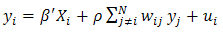
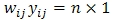
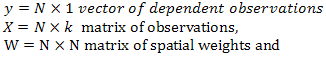
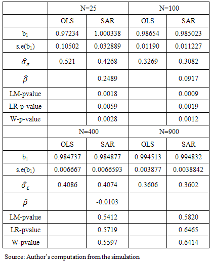
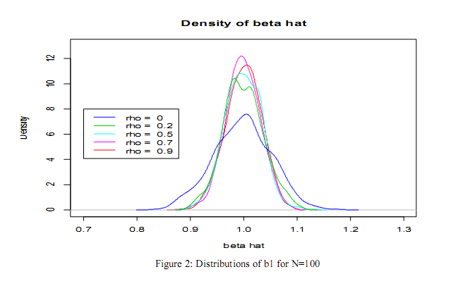
The finding from this study shows that the density of is peakest at a high level of the spatial effect parameter. Therefore the bias becomes larger as the spatial effect parameter increases. This implies that the bias resulting from omitting spatial effect in SAR model is a function of degree or magnitude of spatial effect in the data. If the spatial effect parameter estimate is negligible, so also will the bias and if the spatial effect parameter estimate is strong so also the bias. See figures 1-4 for details.

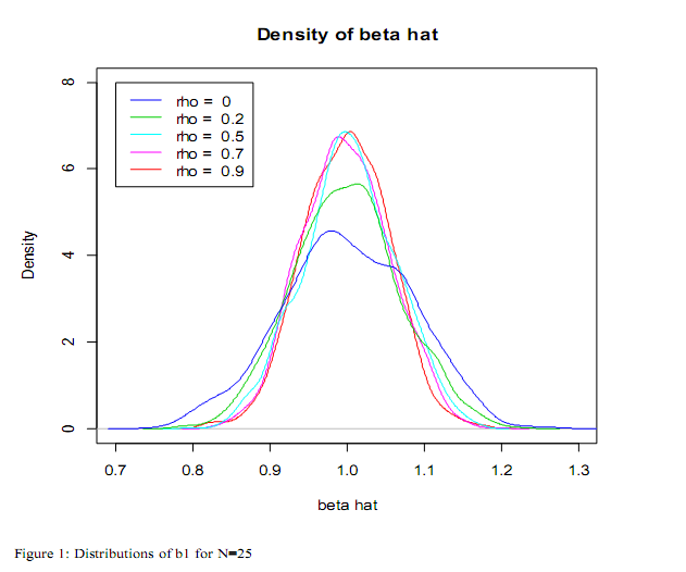Figure 1. Distributions of b1 for N=25

Figure 2. Distributions of b1 for N=100

Figure 3. Distributions of b1 for N=400

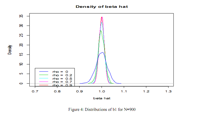Figure 4. Distributions of b1 for N=900

5. Concluding Remarks

This study shows the significance of using the spatial autoregressive model (SAR) when spatial autocorrelation exist in a data set. Spatial econometrics methods allow us to account for dependence between observations, which often arise when observations are collected from points or regions located in space.

The present study shows that the use of OLS to estimate the SAR model is not appropriate because the spatial lag is correlated with the error term and the included explanatory variable. Thus, OLS will produce biased and inconsistent estimate. Findings show that the spatial model performs better than non-spatial model because a lesser error variance was produced in the spatial model in comparison to the non-spatial model.

The study discovered that spatial autocorrelation exists in cases where N=25 and 1000 and the SAR results were significantly different from their OLS counterpart. The smaller error variance in these cases signifies that the SAR model outperforms the OLS (non-spatial) model. The test-statistic values of LM, LR and Wald diagnostic tests for presence spatial dependence in the dataset are not significant hence the parameter estimate of spatial model are not different from their OLS counterparts. In addition, the study established the existence of relationship between bias resulting from omitting spatial effect in SAR model and the magnitude of spatial autocorrelation.

Thus, the SAR model is recommended when spatial diagnostics show the presence of spatial autocorrelation in a dataset. The use of a spatial model if spatial autocorrelation is absent in a dataset results in waste of time and resources.