1. Introduction

Kruskal and Wallis (1952) introduced a rank-based test for comparison of several medians or means, complementing the parametric approaches. Kruskal-Wallis (KW) test is to be among the most useful of available hypothesis testing procedures for behavioural and social research, though it is also one of the many under-utilized nonparametric procedures. Parametric methods, along with the requirement for a stronger set of assumptions, continue to dominate the research landscape despite convincing studies that call into question the wisdom of making such assumptions; see, [2], and [3]. Replacing original scores with ranks does not inherently lead to lower power, as one might suppose, but rather can result in a power increase at best and a slight power loss, at worst; see, for example, [4], [5], [6], [7] and [8].

Kruskal and Wallis [1] said that “...One of the most important applications of the test is in detecting differences among the population means” (p.584). Also they suggested that “… in practice the H test may be fairly insensitive to differences in variability, and so may be useful in the important ‘Behrens-Fisher problem’ of comparing means without assuming equality of variances” (p.599). Furthermore, Iman [9] formulated the null hypothesis of Kurskal-Wallis test in terms of the expected values (p. 726).

When the null hypothesis is rejected, at least one sample stochastically dominates at least another one. The KW test does not identify where this stochastic dominance occurs. Therefore, the Kruskal-Wallis test is rewritten in the form of the sum of independent chi square random variables. Using the idea of Bonferonni approximation, a decision limit for Kruskal-Wallis test is obtained based on the gamma distribution that shows graphically which groups out of the decision limit. A simulation study is conducted using the normal and exponential distributions to confirm the validity and robustness of the decision limit in small and large samples for the new method in comparison with KW test.

The graphical presentation of the KW test is introduced in Section 2. Simulation results to compare between the KW test and the new method are given in Section 3. An application is presented in Section 4. Section 5 is devoted for conclusion.

2. Graphical Presentation of Kruskal-Wallis Test

Suppose independent random observations are obtained from a continuous population with mean and variance is the number of groups or treatments and is the sample size in each group. The model is

is the global location of the data, the difference to the location of the group and is the residual error; see, for example, [2]. Thus the null hypothesis can be expressed as

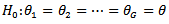versus at least two medians or means are not equal.

2.1. Kruskal-Wallis test

The ranks of the observations are

The Kruskal-Wallis test is defined as

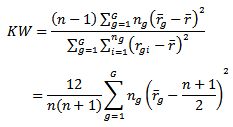where and and it is assumed that the ties are handled by random method.

This is distributed as See, [10] and [1] and [11]. Also, can be written as

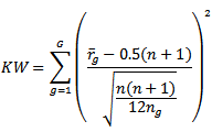The contribution of each standardized group mean rank in the test is defined as

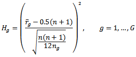Therefore, the Kruskal-Wallis test could be plotted as

This is called H-graph. To do this the sampling distribution of is needed. The first thinking is gamma distribution where [1] used in small sample sizes and the chi square is a special case from it.

2.2. Sampling Distribution of

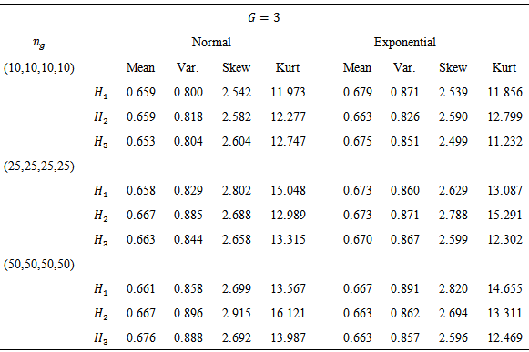
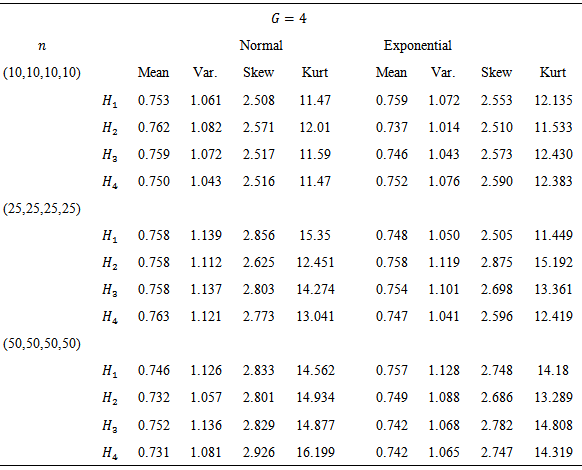
To investigate if the sampling distribution of is a gamma distribution or not, a simulation study is conducted to obtain the first four moments of for and using simulated data from normal and exponential distributions with different sample sizes. Three sets of data are investigated (a) small (b) medium and large The following steps are used in simulation:

1. Simulate data from a distribution with the same mean for the required design.

2. Rank the combined sample, compute for each group and moments for each

3. Repeat this times and compute average for each moments.

Tables 1 and 2 gives the moments of for and

From Tables 1 and 2 it can conclude that

Table 1. Empirical first four moments (mean, variance, skewness and kurtosis) of Hg using simulated data from normal and exponential distributions, G = 3 and the number of replications is 10000

Table 2. Empirical first four moments (mean, variance, skewness and kurtosis) of Hg using simulated data from normal and exponential distributions, G = 4 and the number of replications is 10000

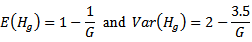
Therefore the chi square distribution with one degree of freedom does not fit for small The gamma distribution is used to fit the sampling distribution of by matching the first two moments; see, [1]. Since the first two moments for gamma distribution are

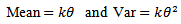where is the shape and is the scale. Therefore,

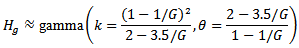Using the shape and the parametrization then

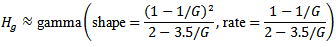It is clear that for large the sampling distribution of approaches chi square distribution with one degree of freedom.

2.3. Graphical Presentation

The Kruskal-Wallis test is plotted as

If any point outside the decision limit, is rejected and this will identify where stochastic dominance occurs.

Since the test is written as sum of independent chi square random variables

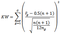and each term has almost the same distribution. Rather than working with whole distribution, it can do the test based on

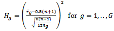with adjusted using Bonferonni approximation. The advantage of this (a) it can tell which group is out of the limit (b) it can easily be used to compute the effect size.

To find the decision limit for there are multiple tests and it is needed to distinguish between two meanings of when performing multiple tests:

1. The probability of making a Type I error when dealing only with a specific test. This probability is denoted (“alpha per test"). It is also called the test-wise alpha.

2. The probability of making at least one Type I error for the whole family of tests. This probability is denoted (“alpha per family of tests”). It is also called the family-wise or the experiment-wise alpha.

The probability of making at least one Type I error for a family of tests is

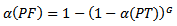This equation can be rewritten as

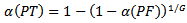For more details; see, for example, [12] and [13].

A simpler approximation which is known as the Bonferonni approximation is

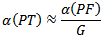For example, to perform and the risk of making at least one Type I error to an overall value of with the Bonferonni approximation, a test reaches significance if its associated probability is smaller than

By using the quantile function of gamma distribution (for example, R-software), the decision limit is

Therefore,

is rejected. Note that this technique is related to analysis of means; see, for example, [14], [15] and [16].

Figure 1 shows the graphical presentation of Kurskal-Wallis test for simulated data from normal and exponential distributions using and total sample sizes 40.

Figures 1 (a) and (c) show the H graph for data simulated from normal and exponential distributions with no shift in mean and it clear that no points outside the decision limit while Figures 1 (b) and (d) show the H graph for data simulated from normal and exponential distributions with shift in mean and is clear that there are points outside the decision limit.

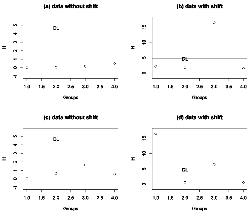Figure 1. H-graph with decision line for G = 4 and n = 40 using simulated data: (a) normal with equal means (100,100,100,100), (b) normal with shift in mean (100,100,90,100), (c) exponential with means (1,1,1,1,1) and (d) exponential with shift in mean (9,1,1,1)

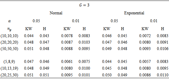
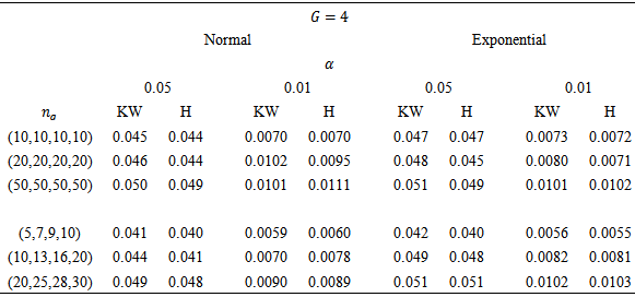
3. Comparisons

The new method is compared with KW test in terms of Type I error. Two variables were manipulated in the study: (a) number of groups (3 and 4) and (b) sample size (small-medium-large). For each design size, three sample size cases were investigated. In our designs, the smallest of the three cases investigated for each design has an average group size of less than 10, the middle has an average group size less than 20 while the larger case in each design had an average group size less than 30. With respect to the effects of distributional shape on Type I error, the normal and exponential distributions were selected.

To evaluate the particular conditions under which a test was insensitive to assumption violations, the idea of [17] of robustness criterion was employed. According to this criterion, in order for a test to be considered robust, its empirical rate of Type I error must be contained in the interval The choice of Bradley was and this makes the interval is liberal. Therefore, in this study the choice of a something in the middle between nothing and 0.025. Therefore, for the five percent level of significance, a test was considered robust in a particular condition if its empirical rate of Type I error fell within the interval and for the one percent level of significance the choice of a test was considered robust if its empirical rate of Type I error fell within the interval . Correspondingly, a test was considered to be nonrobust if, for a particular condition, its Type I error rate was not contained in these intervals. Nonetheless, there is no one universal standard by which tests are judged to be robust, so different interpretations of the results are possible.

Tables 3 and 4 contain empirical rates of Type I error for a design containing three and four groups, respectively. The tabled data indicates that

1. When the observations were obtained from normal distributions, rates of Type I error were controlled by KW and H methods for equal and non equal sample sizes.

2. When the observations were obtained from non-normal distributions, rates of Type I error were controlled by KW and H methods for equal and non equal sample sizes.

Table 3. Empirical Type I error for Kruskal-Wallis (KW) and Hg tests for G = 3 using simulated data from normal and exponential distributions and the number of replications is 10000

Table 4. Empirical Type I error for Kruskal-Wallis (KW) and Hg tests for G = 4 using simulated data from normal and exponential distributions and the number of replications is 10000

4. Application

From [18] a study of the use of a semi automated method for measuring the amount of chlopheniramine maleate in tablets, for each of four manufacturers, composites were prepared by grinding and mixing together tablets that had nominal dosage levels of 4 mg. Seven labs were asked to make 10 determinations on each composite; each determination was made on a portion of composite whose weight was equivalent to that of one tablet. The purpose of the experiment: are the differences in the means or medians of the measurement from the various labs significant, or might they be due to chances?

Table 5 gives the amount of chlopheniramine maleate in tablets for seven labs.

Table 5. The amount of chlopheniramine maleate in tablets for seven labs

Using the Kruskal-Wallis it is found that

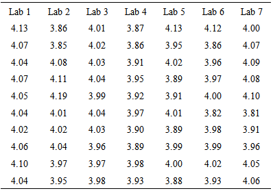
This indicates that there is a systematic difference among the labs at 0.05 and 0.01 level of significance without telling anything about the differences.

While H-graph in Figure 2 shows that there are two points outside the decision limit that indicates there is a systematic difference among the labs at 0.05 and 0.01 level of significance. Moreover identify the labs 1 and 4 as different from the overall mean.

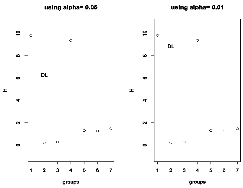Figure 2. H-graph for the amount of chlopheniramine maleate in tablet data

5. Conclusions

A graphical presentation of Kruskal Wallis test is studied by re-expressing the test as sum of independent chi square random variables. The sampling distribution for this function was obtained and found that the gamma distribution had given a very good fit for this function until for small sample sizes.

A decision limit is obtained using the gamma distribution and Bonferonni approximation that enabled us to show Kruskal-Wallis test graphically. The main advantage of the new method is not only provided us about the differences in medians or means but also where these differences had been happened. Moreover, a simulation study confirmed the validity and robustness of the decision limit in small and large samples in comparison with Kruskal Wallis test.