Usoro Anthony Effiong
Department of Mathematics and Statistics, Akwa Ibom State University, Mkpat Enin, Nigeria
Correspondence to: Usoro Anthony Effiong, Department of Mathematics and Statistics, Akwa Ibom State University, Mkpat Enin, Nigeria.
| Email: |  |
Copyright © 2015 Scientific & Academic Publishing. All Rights Reserved.
Abstract
This paper considered estimation of long-range parameters of a seasonal model using regression approach. Multiple linear regression model was deduced from SARIMA (5, 0, 0)x(0, 1, 0)4 model. The data used were quarterly data of Nigerian gross domestic products from 1997 to 2012, CBN Statistical Bulletin, 2012(x106). The Multiple linear regression model was fitted to the data, and the necessary diagnostic check through ACF and PACF revealed model reliability. From the model, forecast function for gross domestic products was obtained. From the basic statistics, the values of the forecast give better results.
Keywords:
SARIMA Model, Multiple Regression, Time Series
Cite this paper: Usoro Anthony Effiong, Estimation of Parameters of Multiplicative Seasonal Autoregressive Integrated Moving Average Model Using Multiple Regression, International Journal of Statistics and Applications, Vol. 5 No. 2, 2015, pp. 91-97. doi: 10.5923/j.statistics.20150502.07.
1. Introduction
Seasonality in a time series is a regular pattern of changes that repeats over S time-periods, where S defines the number of time-periods until the pattern repeats again. For example, there is seasonality in monthly data for which high values tend always to occur in some particular months and low values tend always to occur in other particular months. In this case, S=12(months per year) is the span of the periodic seasonal behaviour. For quarterly data, S=4 time periods per year. A seasonal ARIMA model or SARIMA model incorporates both non-seasonal and seasonal factors in a multiplicative model. One shorthand notation for the model isSARIMA (p, d, q)x(P, D, Q)s, with p=non-seasonal AR order, d=non-seasonal differencing, q=non-seasonal MA order, P=seasonal AR order, D=seasonal differencing, Q=seasonal MA order, and S=time span of repeating seasonal pattern. The above model is, | (1) |
The non-seasonal components are: | (2) |
 | (3) |
The seasonal components are: | (4) |
 | (5) |
In the left hand side of the equation ‘1’, the seasonal and non-seasonal AR components multiply each other, and on the right hand side, the seasonal and non-seasonal MA components multiply each other [16].In statistics, linear regression is an approach for modelling the relationship between a scalar dependent variable y and one or more explanatory variables (or independent variable) denoted X. A case of one explanatory variable is Simple Linear Regression. For more than one explanatory variable, it becomes Multiple Linear Regression, [5]. In linear regression, data are modelled using linear predictor functions, and unknown model parameters. Such models are linear models [8]. Linear regression was the first type of regression analysis studied rigorously and extensively in practical applications [20]. Linear regression has many practical uses. Most applications fall into one of the following two broad categories; prediction/forecasting and measuring the strength of relationship between the dependent and independent variables. In statistics and econometrics, a distributed lag model is a model for time series data in which a regression equation is used to predict current values of a dependent variable based on both the current and lagged (past period) values of an explanatory variable, [9]. The simplest way to estimate parameters associated with distributed lags is by ordinary least squares, assuming a fixed maximum lag p, assuming identically independently distributed errors [10].In time series, if there are long-range parameters, it becomes easier to estimate the parameters associated with the distributed lags of the dependent variables using regression method. This is a case of univariate time series, and the model is autoregressive model. If the distributed variables include both the dependent and independent variables, the model becomes multivariate time series model, [17]. Many researchers have used regression approach to estimate parameters of time series model with both short range and long-range dependence. Long Range Dependence, also called long memory or long- range persistence, is a phenomenon that may arise in the spatial or time series data. It relates to the rate of statistical dependence, with the implication that this decays more slowly than an exponential decay, typically a power-like decay. LRD has application in various fields, such as internet traffic modelling, econometrics, hydrology, linguistics and the earth sciences, (Wikipedia, the free encyclopedia). Different mathematical definitions of LRD are used for different context and purposes, [2], [7], [15], [3], [18], [13]. [14] carried out log–periodogram regression of time series with long-range dependence. The paper discussed the estimation of multiple time series models, which allow elements of the spectral density matrix to tend to infinity or zero. A form of log-periodogram regression estimate of differencing and scale parameters was proposed, which according to the paper, can provide modest efficiency improvements over a previously proposed method (for which no satisfactory theoretical justification seems previously available) and further improvements in a multivariate context when differencing parameters are a priori equal. [1] proposed statistical methods for data with long-range dependence. [6] obtained efficient location and regression estimation for long-range dependence regression models. [11] obtained M-estimators in linear models with long-range dependence errors. [19] estimated a regression model with long memory stationary errors. [12] estimated parameters in linear regression with long-range dependence errors. [21] modelled long memory time series. In time series modelling, it is very common that the order of stationary time series model is always limited to maximum of order 2. This is evident in most of the research works and publications in the areas of time series. This does not negate the fact that parameterization may be necessary in some cases to completely specify a model. Parameterization means the process of deciding and defining the parameters necessary for a complete or relevant specification of a model. Sometimes, a model with short-range dependence may need possible extension to accommodate more parameters. This paper intends to apply the reduced form of the regression variables to estimate the parameters of the SARIMA models with long-range dependence in the form of multiple linear regression model, so as to check if the deduced regression model has compared favourably with the direct method of estimating multiplicative SARIMA model.
2. Method
The initial investigation requires the application of [4] methodology. For proper identification and choice of a model, plots of the original, differenced series, ACF and PACF are necessary.Graphs ‘1’ and ‘2’ are the plots of the original and differenced Xt series.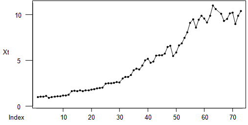 | Graph 1. Plot of the original Xt |
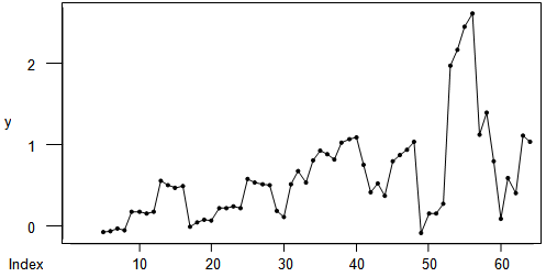 | Graph 2. Plot of the differenced Xt |
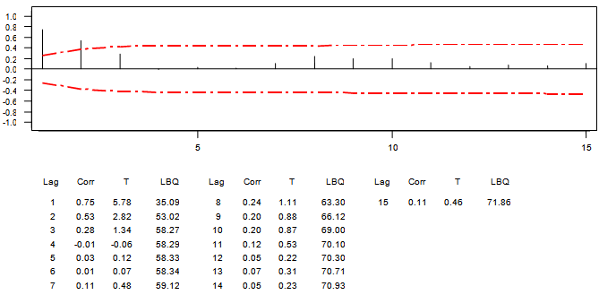
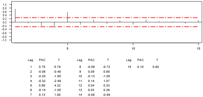
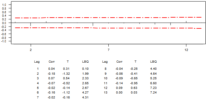
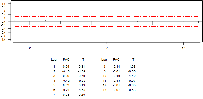
The above ACF and PACF of the first order seasonal differenced series suggest SARIMA (5, 0, 0) x (0, 1,0)4. The model is specified with long-range parameters because the PACF values are significant up to lag 5, and insignificant from the sixth lag. The ACF show gradual decay in its values from the first lag to subsequent lags. The model requires parameterization (increase in the number of parameters up to the fifth lag due to the significant effect of the PACF at lag 5). The general form of the model is, | (6) |
The above model is expanded as follows,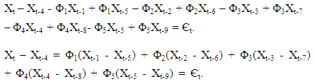 | (7) |
Let Xt – Xt-4 = Yt, Xt-1 – Xt-5 = Yt-1, Xt-2 – Xt-6 = Yt-3, Xt-4 – Xt-8 = Yt-4, Xt-5 – Xt-9 = Yt-5.Equation ‘7’ reduces to  | (8) |
Equation ‘8’ is a multiple linear regression model with the lags of Yt as the independent variables, while Yt is the dependent variable. The usual assumption  .
.  | Graph 3. ACF of the Differenced Series (DXt) |
 | Graph 4. Plot PACF of the differenced Series DXt |
3. Analyses and Results
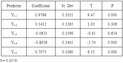
The regression of Yt on Yt-1, Yt-2, Yt-3, Yt-4, and Yt-5 produces the following parameter estimates for the predictive model of Yt, | (9) |
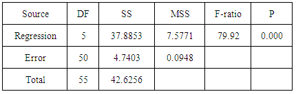
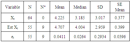
Equation ‘9’ is the predictive model of ‘8’. The parameters of the model lie within unit circle. This implies there is no violation of invertibility condition of a stationary time series. The regression estimates in Table’1’ indicate the significant effect of Yt-1, Yt-4 and Yt-5. This further justifies the parameterization of the model to include up to the fifth lagged variable. Analysis of variance, as shown in Table ‘2’ indicates overall fitness of the model into the data. Table ‘3’ presents the basic statistics of the actual, estimated values of Xt and as well as residual values. This clearly shows that the assumption of the error is not violated, as the mean is approximately zero with minimum standard deviation. In addition, the model has given good estimates compared to the actual values. Evidence is shown in Table ‘4’and graph ‘5’.Table 1. Regression Estimates
 |
| |
|
Table 2. Analysis of Variance
 |
| |
|
Table 3. Basic Statistics
 |
| |
|
Table 4. Original and Estimated values of Xt
 |
| |
|
Apart from the basic statistics of the error values displayed in Table ‘3’, the analysis requires further explanation about the behaviour of the error values after estimation of the model parameters. The ACF and PACF as shown in Graphs ‘6’ and ‘7’ were necessary to check for the distribution of the error. It is evident that the error 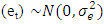 .
.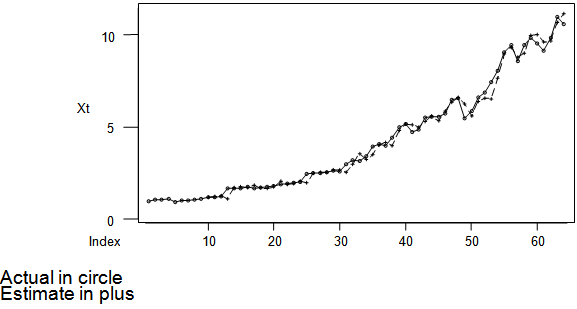 | Graph 5. Plot of actual and estimated values |
 | Graph 6. ACF of the Residual |
 | Graph 7. PACF of the Residual |
4. Forecasts
Equation ‘9’ is the estimated model of equation ‘8’. This is the reduced form of equation ‘7’. By substitution, the equation ‘7’ becomesXt – Xt-4 = 0.98(Xt-1 - Xt-5) + 0.1412(Xt-2 - Xt-6) – 0.0631(Xt-3 - Xt-7) – 0.8058(Xt-4-Xt-8) + 0.7073(Xt-5 - Xt-9) = 0.980Xt-1 + 0.1412Xt-2 – 0.0631Xt-3 + 0.1942Xt-4 – 0.2727Xt-5 – 0.1412Xt-6 + 0.0631Xt-7 + 0.8058Xt-8 – 0.7073Xt-9.The forecast equation is given by,
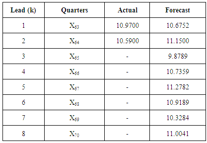
 = 0.980Xt+k-1 + 0.1412Xt+k-2 – 0.0631Xt+k-3 + 0.1942Xt+k-4 – 0.2727Xt+k-5 – 0.1412Xt+k-6 + 0.0631Xt+k-7 + 0.8058Xt+k-8 – 0.7073Xt+k-9Where t is the time for each forecast, k is the lead time.
 Table 5. Quarterly Forecast of Nigerian Gross Domestic Products
 |
| |
|
5. Summary and Conclusions
The method of modelling in this paper is not at variance with [4] approach to time series modelling. Preliminary investigation was carried out with the plots of ACF and PACF for proper choice of the model. The ACF and PACF of the first order differencing suggested SARIMA (5, 0, 0) X(0, 1, 0). This implies that the PACF of the seasonally differenced series exhibited significant cut off up to the fifth lag, and became insignificant from the sixth lag to the last. Parameterization was required in the choice of the model. With the parameterization, there was a long-range dependence on the parameters. The objective was to reduce the model to a multiple linear regression model, whose parameters can be estimated with ordinary least squares method. The reduced form of the model included Yt-1, Yt-2, Yt-3, Yt-4 and Yt-5 lagged variables of the observed time series variable Yt, with associated parameters Φ1, Φ2, Φ3, Φ4 and Φ5 respectively. The parameters of the regression model were estimated, and the estimates obtained from the fitted model are compared favourably with the actual values of the gross domestic products (see graph 5). Diagnostic check through the ACF and PACF of the residual values is a clear indication that there is much improvement in this model and approach adopted on the previously proposed models for Nigerian Gross Domestic Products. The values of the forecast obtained from the model are more accurate and reliable planning purposes.
References
| [1] | Beran, Jan. (1992): Statistical methods for data with long range dependence. Statistical Science 7, pp 404-1047. |
| [2] | Beran, Jan (1994): Statistics for Long Memory Processes. CRC press. |
| [3] | Beran et al. (2013): Long memory processes: Probabilistic Properties and Statistical methods. Springer. |
| [4] | Box, G. E. P. And Jenkins, G. M. (1976): Time Series Analysis; Forecasting and Control 1st Edition, Holden-day, san Francisco. |
| [5] | David A. Freedman (2009): Statistical Models; Theory and Practice, Cambridge University Press p.26. |
| [6] | Dahihaus, R. (1995): Efficient location and regression estimation for long range dependence regression models. Annals of Statistics 23, pp1029-1047. |
| [7] | Doukhan et al. (2003): Theory and Applications of Long Range Dependence. Birkhäuser |
| [8] | Hilary L. Seal (1967): The Historical development of the Gauss Linear model. Biometrika 54(1/2): 1-24. |
| [9] | Jeff B. Cromwell, et al (1994): Multivariate Test for Time Series Models. SAGE publications, Inc ISBN 0-8039-5440-9. |
| [10] | Judge, George, et al (1980): The theory and practice of Econometrics, Wiley Publications. |
| [11] | Koul, H. L. (1992): M-estimators in linear models with long-range dependence errors. Statistics Probability Letters, 14, pp. 153-164. |
| [12] | Liudas Giraitis and Hira Koul (1997): Estimation of the dependence parameters in linear regression with long range dependence errors. Stochastic Process and their Applications Vol. 71, Issue 2, pp 207-224. Elsevier doi:10.1016/S0304-4149(97)00061-6. |
| [13] | Malamud, Bruce D. And Turcotte, Donald L. (1999): ‘Self-Affine Time Series. I. Generation and Analyses’. Advances in Geophysics 40: 1-90. doi:10.1016/S0065-2687(08)60293-9. |
| [14] | Robinson, P. M. (1995): Log-Periodogram Regression of Time Series with Long Range Dependence. The Annals of Statistics. Volume 23, No.3, pp.1048-1072. |
| [15] | Samorodnitsky, Gennady (2007): Long range dependence. Foundation and Trends in Stochastic Systems. |
| [16] | Https://onlinecourses.science.psu.edu/stat 510/node/67. |
| [17] | Usoro, A. E and Omekara, C. O (2008): Bilinear Autoregressive Vector Models and their Application to Revenue Series. Asian Journal of Mathematics and Statistics 1(1): 50-56. |
| [18] | Witt, Annette and Malamud, Bruce D. (2013):’Quantification of Long-Range Persistence in Geophysical Time Series; Conventional and Benchmark-Based Improvement Techniques’. Surveys in Geophysics (springer) 34(5):51-651. doi:10.1007/S10712-012-9217-8. |
| [19] | Yajma, Y. (1988): On estimation of a regression model with long memory stationary errors. Annals of Statistics 16, pp 791-807. |
| [20] | Yan, Xin (2009): Linear Regression Analysis: Theory and Computing. World Scientific, pp. 1-2. |
| [21] | Yushihiro Yajima (1985): On the estimation of long memory time series models. Australian Journal of Statistics, Vol. 27 Issue3, pp303-320. |
 Abstract
 Reference
 Full-Text PDF
 Full-text HTML