Lawal Ganiyu Omoniyi , Aweda Nurudeen Olawale
Department of Statistics, Yaba College of Technology, Nigeria
Correspondence to: Aweda Nurudeen Olawale , Department of Statistics, Yaba College of Technology, Nigeria.
| Email: |  |
Copyright © 2015 Scientific & Academic Publishing. All Rights Reserved.
Abstract
Bounds testing procedure is a powerful statistical tool in the estimation of level relationships when the underlying property of time series is entirely I(0), entirely I(1) or jointly cointegrated. A univariate framework for testing the existence of single level relationship between exchange rate, crude oil prices and inflation rate in Nigeria was postulated using ARDL (4,4,0) model in this paper. Bound testing as an extension of ARDL modelling uses F and t-statistics to test the significance of the lagged levels of the variables in a univariate equilibrium correction system when it is unclear if the data generating process underlying a time series is trend or first difference stationary. Empirical analysis shows that these macroeconomic variables have highly significant level relationship with exchange rate irrespective of the underlying properties of their series. The conditional level relationship model and the associated conditional unrestricted equilibrium correction model (ECM) in the long- and short-run relate crude oil prices negatively and inflation rate positively with exchange rate. The long run speed of adjustment to equilibrium reveals that exchange rate in Nigeria is slow to react to shocks on crude oil prices and inflation rate.
Keywords:
Bounds testing, ARDL, Cointegrated, Conditional unrestricted equilibrium correction model (ECM), Conditional level relationship model, Exchange rate, Crude oil prices, and inflation rate
Cite this paper: Lawal Ganiyu Omoniyi , Aweda Nurudeen Olawale , An Application of ARDL Bounds Testing Procedure to the Estimation of Level Relationship between Exchange Rate, Crude Oil Price and Inflation Rate in Nigeria, International Journal of Statistics and Applications, Vol. 5 No. 2, 2015, pp. 81-90. doi: 10.5923/j.statistics.20150502.06.
1. Introduction
Exchange rate movement and its impact on the Nigerian economy have received some attention over the years. Exchange rate is the value of a country`s currency in terms of another currency (US dollars as base currency in the case of Nigeria). This macroeconomic variable plays a major role in the stability of any economy. Productivity of a country is enhanced through stable currency by keeping costs and prices of goods and services as low as possible. Several factors are responsible for the determination of exchange rate; levels of prices, interest rates movements, current account deficit, and level of public debt, balance of payment position, political stability and economic performance are few of these factors. In Nigeria, the national output measured (mainly by the gross domestic product (GDP)) predominantly revenue from crude oil export continues to play a major role in the determination of the country’s current account deficit, level of public debts, balance of payments, monetary and fiscal policy, and to a large extent the political stability. Since her independence in 1960, revenues from the sales of crude oil have continued to rise leading to an import dependent production structure, weak production and fragile export base. Furthermore revenues from sales of crude oil determine largely the federal and states budget projections based on a benched mark crude oil price. Therefore, the linkage between exchange rate and crude oil prices cannot be overlooked. For example, [1] iterated that appreciation of the real exchange rate is caused by increase in non-tradable goods as a result of rising cost of production which stems from crude oil price increase. However, rise in crude oil prices have negative effect on the purchasing power of the consumers of non-tradable goods. This will result in the fall of the demand and eventually social prices of these goods. Exchange rate divergences directly have an impact on the social output prices and the cost of production. The effect of exchange rate depreciation on production of social/ nontradeable goods is negative due to forces such as deflationary policy which creates sustainable production equilibrium for the economy through reduced government spending, higher taxes, and higher interest rates. In South Africa, the fundamental relationship between exchange rate and crude oil prices is such that higher crude oil prices results in depreciation of the South African rand which can cause a major misalignment in the local currency [2]. By using cointegration analysis, [3] established a positive relationship between real crude oil price and real exchange rate in Nigeria. They associated the bubble in real exchange rate between 2000 and 2010 with rise in real crude oil prices. [4] using the Johansen method of cointegration in studying the causal relationships between exchange rate, crude oil price, and commodity prices in United States concluded that rise in crude oil prices have significant negative causal effects on exchange rate both in the long- and short-run in the United States. By conducting a panel data analysis on 65 oil importing countries, [5] found out that depreciation of local currency against the US dollar is directly linked to the rise in the crude oil demand which was larger than the effect the movement in crude prices had on exchange rate in those countries. Similarly, [6] in her working paper which employed panel data analysis on 33 oil exporting countries concluded that real exchange rate and crude oil price cointegrated in those countries with sound bureaucratic and impartial legal systems. [7] showed that there exist a significant negative relationship between the crude oil price and real exchange rate in the United Arab Emirates by employing the vector error correction model proposed by [8]. Crude oil price and price level in an economy are linked in a cause and effect relationship. As discussed earlier, crude oil prices determine the production cost which in turn has a direct effect on the prices of goods in the country. Lower inflation rates tend to improve the value of the local currency due to the fact that purchasing power of the currency increases relative to other currencies. Theoretically, purchasing power parity establishes the link between exchange rate and the inflation or relative prices of goods. Hence equilibrium exists between two currencies if purchasing powers at a rate of exchange are equivalent. Many developed countries are known to have low inflation rates and therefore have enjoyed an appreciating currency unlike countries with high inflation rates. Therefore, for heavily export oriented economy, it is expected that rising inflation will lead to higher exchange rate. Hence, higher inflation depreciates the value of the local currency. However, fixed nominal exchange rate is an effective shock absorber to inflationary pressure in countries practising the inflation targeting1 monetary policy [9]. The aim of this paper is to establish a level relationship between exchange rate, crude oil prices and inflation rate by employing the Autoregressive Distributed-Lag (ARDL, hereon) Bounds testing approach proposed by [10] under a conditional equilibrium correction model (ECM) framework.
2. Source of Data
The data employed in this paper are monthly time series data of exchange rate(er), crude oil prices (cp), and inflation rates (ir). All data are sourced from the statistical database of the Central Bank of Nigeria (CBN). Monthly data from 2004 to 2014 were extracted and analysed by building ARDL (p, p1, p2) model. All data were transformed to log so that they have same magnitude and to improve the data analysis.
3. Empirical Data Analysis and Results
In order to study the relationships between exchange rate and two very important factors influencing its movement in Nigeria, an empirical application of the bounds testing proposed by [10] was established.
4. Unit Root Tests – Augmented Dickey-Fuller (ADF) Tests
The underlying properties of the time series were established by testing for the existence of unit roots using mainly the methods proposed by [11]. All variables were assumed to follow a random walk or are non-stationary based on the individual series time plot in Figure 1.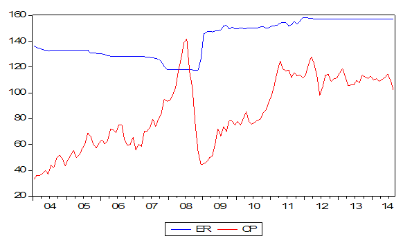 | Figure 1. Time Series Plots on Exchange rate, crude oil price |
Since it is important (though not necessary since the bounds testing procedure presume that there exists a level relationship irrespective of the order of integration of the variables) to determine the underlying properties of processes that generated the data particularly when modelling long run relationships in time series analysis, further tests of unit root were conducted. This is essential if we are to avoid the problem of spurious regression (associated with stochastic or random trends imminent in the data) usually encountered when non stationary series/random walks are “regressed” against each other producing a statistically significant long run relationships inform of contemporaneous correlations. However, since the object is to produce meaningful causal relations in this research work we conducted unit roots test employing the Augmented Dickey-Fuller test procedure on the macroeconomic variables. The ADF test is an extension of [12] procedure, which uses a t-ratio test statistic. A major difference between the two procedures is that ADF requires additional extra lagged terms of the dependent variable in the test equation. We begin unit root tests by reviewing Dickey-Fuller test involving a simple AR(1) process, then the more complicated Augmented Dickey-Fuller test involving ARMA(p,q) process. Dickey-Fuller test statistic centres on the DF distribution of the t- ratio statistic of (ø1 – 1)/σ(ø1) whereby ø1 and σe are the Least Squares estimates of ø1 and σe respectively derived from the estimation of the simple models 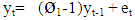 | (1.1) |
The test hypothesis is: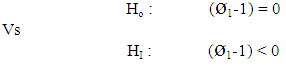
 | Figure 2. Time Series Plots on Inflation Rates |
The critical values of the t-ratio in 1.1 was based on DF τ- distribution rather than the standard t-distribution in order to avoid the over rejection of null hypothesis. Equation1.1 assumes that the overall mean of the series is zero which imply that there is no deterministic term in the AR(1) process and yt is equal to zero at t= 0. Since, we do not know whether y0 is equal to zero, a deterministic term λ was allowed to enter the model for the purpose of unit root testing. A reparameterized equation 1.1 is given as: | (1.2) |
et is independently and identically distributed DF with mean zero and variance σ2. Also, if yt contains stochastic trend, we introduce a time trend t in equation 1.2 above and test for the unit root. The null hypothesis is one of series contain stochastic trend against an alternative of trend stationarity. The equation of regression becomes: | (1.3) |
However, yt may contain both an autoregressive AR(p) and moving average MA(q) processes making the test of unit roots more complicated. In this case et will be autocorrelated. [11] augmented the DF test to accommodate ARMA (p, q) models with unknown orders using the regression with various assumptions about the data generating process:• No trend and no intercept  | (1.4) |
• Intercept but no trend | (1.5) |
• Intercept and trend | (1.6) |
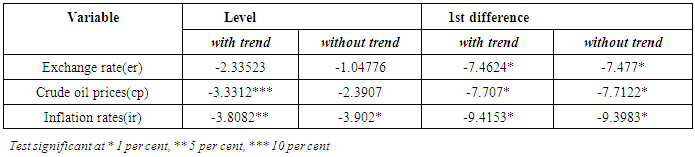
Where φ* = (φ1+ φ2 + φ3 + .......+ φp)-1, et independently and identically distributed dickey-fuller with mean zero and variance σ2. The test of hypothesis is φ*=0 against φ*<0 which is based on the test of DF statistics φ*/SE (φ*). Equation 1.6 point to the fact that a time series is stationary around a deterministic time trend which may result in a permanent shift in the mean and trend during the review period.From the Table 1, it can be observed that only exchange rate is integrated of order one. Whilst crude oil prices is trend stationary, inflation rates is considered to be a stationary series. The mixed results of unit root tests above indicate that there might be no level relationship between the three variables. Using the Bounds testing procedure proposed by [10], we test for the existence of level relationships between the variables regardless of whether they are integrated of order one or zero or mutually cointegrated. Having established the underlying properties of the time series variables in the study based on the ADF test results, an unrestricted equilibrium correction model was developed to study the long-run and short-run causal relationships between exchange rate and the other two macroeconomic variables. Table 1. Unit root tests- ADF
 |
| |
|
5. Test of Granger Causality between Exchange Rate, Crude Oil Prices and Inflation Rate
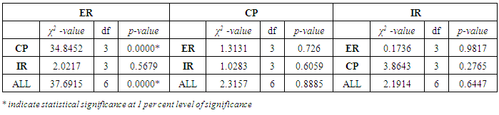
An initial test of granger causality between variables using the procedure proposed by [13] was conducted. Since the presence of nuisance parameter in the VAR invalidates the popular Wald test statistic, they showed that under null hypothesis, the linear restrictions on parameters of a VAR model where some of the series are non-stationary would not follow the usual asymptotic chi-square distribution [14].This method involves testing for the absence of Granger causality by testing the null hypotheses of X does not Granger-cause Y and vice versa2. If these null hypotheses are rejected in both cases, this implies that there exists Granger causality. Granger non-causality test results (Table 2) show that there exists unidirectional causality from crude oil prices to exchange rate. However, crude oil prices and inflation rates considered together granger causes exchange rate though inflation rate remain highly insignificant in determining the future values of exchange rate in Nigeria. This will further be revealed later in the conditional long-run relationships between this variables. Hence using exchange rate as the dependent variable in the dynamic ARDL model was further justified.Table 2. Granger Causality between exchange rate, crude oil price, Inflation rate
 |
| |
|
6. Test of Cointegration Using Autoregressive Distributed-lag (ARDL) Bounds Testing Approach
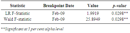
Autoregressive distributed-lag models (ARDL model, hereon) are widely employed in the analysis of long-run relations when the data generating process underlying the time series is integrated of order one (i.e. I(1)). Recently, the application of ARDL model procedure to difference- stationary series has been evolving. One of the earliest work in this area was done by [15] who proved that when the underlying data generating process of time series is I(1), the Ordinary Least Squares (OLS, hereon)parameter estimators in the short-run are 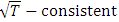 where T is the sample size. Bound testing as an extension of ARDL modelling uses F and t-statistics to test the significance of the lagged levels of the variables in a univariate error correction system when it is unclear if the data generating process underlying a time series is trend or first difference stationary [10]. Prior to this method of cointegration, several techniques have been proposed in establishing cointegrating relations amongst nonstationary time series. Prominent are the works of [16], [8], [17]. Bounds testing is preferred to these other methods due to its relative better performance when the sample size T is small and its applicability to a mixture of stationary and non-stationary time series. [10] proposed several consistent bounds testing procedure which follow asymptotic distribution. In this research work, we approximated the time series properties of exchange rate, crude oil prices and inflation rate by a log-linear VAR(p) model (equation 1.7), incorporating deterministic terms such as intercept and time trends. This is important to improve the interpretability of model coefficients and to address the issue of outliers by ensuring that the variables are normally distributed. Also, one dummy variable (which does not modify the asymptotic property of both Wald and F-statistic) was introduced in the model to capture structural breaks resulting from crash in global crude oil price in 2009. This date was computed using the constancy of parameter procedure proposed by [18] with 49 per cent data trimming3. The result is as shown in Table 3. We defined the dummy variable as
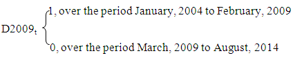 Notice that as T - ∞, the number of non-zero entries approaches zero. Therefore, the asymptotic properties of the Wald and F-statistic in the bounds test remained unaffected. The introduction of this one off dummy variable was to deal with problem of over acceptance of the null hypothesis under ADF test which may result in an increased type II error or reduced power of the test
Table 3. Quandt Andrews Breakpoint Test
 |
| |
|
7. Unrestricted VAR(p) Exchange Rate Model
We postulated a VAR(p) model with unrestricted deterministic terms and dummy variable as follows: | (1.7) |
where | (1.8) |
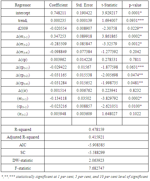
zt =(yt, xt′)′ = (ert, cpt′, ir′t)′. By partitioning the error term εt in 1.8 appropriately with zt, we have α0= (αy0, α′x0)′, α1 = (αy1, α′x1)′ , ∏= (πy, ∏′x)′, Γ = (γyi, Γ′x)′. Given that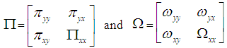 c0=-(πyy, πyx.x)μ + [γy.x + (πyy, πyx.x)]γ, c1 = -(πyy, πyx.x)γ, πyx.x = πyx - ω′ ∏xx, and ψ′i = γyi - ω′ Γxi , i = 1,2,3,.......,p-1, ut are serially uncorrelated disturbances. ∆xt are uncorrelated with disturbances ut. Since the disturbances in equation 1.7 are serially uncorrelated with mean zero and variance (Ω), the selection of an appropriate lag order for the model is essential. The proper choice of the lag order p is such that it is neither too small nor too large. If small, the variables not included in the model will be accounted for in the disturbances thereby leading to residual serial correlation problem. Contrarily, if the p is large, this will result in over-parameterisation of the model with small sample size. Hence, this research work uses the Bayes Criterion also referred to as Schwarz Criterion (SC, hereon)4 because of its consistency as model selector, details of which is outside the scope of this current work. SC alongside the Akaike information criteria selected a p=4 for the VAR model in 1.7. This maximum lag was chosen after comparing the AIC (-5.9084) and SC (-5.5883) values for p=4 with p = 1 , 2 , 3, 5 and 6 at the same time ensuring that the residuals remain uncorrelated by conducting a Lagrange Multiplier test on each model. The lagged first difference variables, ∆irt-1, ∆irt-2........ are statistically insignificant in all the models postulated, hence were removed from the analysis to forestall the problem of over-parameterization of the conditional equilibrium correction model in equation 1.7. This further explains why the past and current values of inflation rates are not significant in the forecast of exchange rate values in the granger causality tests. The model in 1.7 above stems from a simple VAR(p) data generating process5 expressed as a vector error correction model6. The lag polynomial Φ(L) can be expressed in an error correction form Φ(L) = -∏L + Γ(L)(1- L) under the assumptions that the characteristics roots given as │Ӏm - ∑Φizi│= 0 lies outside the unit circle │z│= 1 [15] and the error terms εt is IN(0,Ω). The former assumption implies that exchange rate(er), crude oil price (cp) and inflation rates (ir) in zt can be purely I(1), I(0) or even cointegrated except for seasonal unit roots and explosive roots i.e I(2) or larger [10]. The results of ADF unit roots test showed that none of the variables are I(2) or more. The partitioning of the disturbances εt with zt = (yt′, xt′)′ as εt = (εyt, ε′xt)′ was done so that εyt can be expressed conditionally in terms of ε′xt in the form εyt = ωyxΩ-1xxεxt + ut where ut are IN(0,ωuu). The model in 1.7 is referred to as a conditional unrestricted equilibrium correction model. We estimated the long-run parameters and their respective standard errors (S.E) using the OLS method under the assumption that the lagged exchange rate, ert-1, does not enter the sub-VAR model for xt. Table 4 shows values of long-run (∏) and short-run (Γi) coefficients along with their standard errors of the initial unrestricted error correction model prior to bounds testing. Constraints were imposed on the intercept and the time trend such that α0 ≡-∏μ + (Γ+∏) γ and α1≡ -∏ γ. As long as the γ ≠ 0, the trend coefficient α1=0.000235 in Table 4 ensure that the deterministic trending behaviour of the level process zt is invariant to the cointegrating rank of the long-run (∏) matrix [10]. The same assertions applies to the intercept α0=0.7482 but γ = 0. Hence a bounds test based on the F-statistics gives similar asymptotic results with Wald statistic which will be shown later in the paper. This unrestricted ECM relates the exchange rate positively with inflation rates and negatively with crude oil prices both in the long- and short-run which are expected according to the literature. Specifically, the long-run coefficients between exchange rate (er) and crude oil prices (cpt-1), exchange rate and inflation rates (irt-1) are -0.1731 and 0.0444 respectively. These values were derived from – (πy.x/πyy) at t-1 and imply that 1 per cent increase in crude oil price will result in 0.1731 per cent decline in the exchange rate. Similarly, 1 per cent increase in the inflation rates will result in about 0.0444 per cent increase in exchange rate in the long run. Shocks on crude oil prices lead to decline of exchange rate or at least create stability in the exchange rate due to growth in foreign reserve7 which is used by the monetary authorities in their monetary policy implementation. However, the Nigerian central bank has been known to practice the inflation targeting policy through interest rates adjustment over the years. Therefore, the significant drop in exchange rate during periods of rising oil prices can be attributable to the fact that Nigeria generates significant earnings from crude oil exports resulting in robust foreign reserve to augment the hugely growing local demands for the US dollars. The inflation rate has no significant short-run relationships with exchange rate probably because the primary purpose of the exchange rate is to stabilize the Naira against the US dollar rather than control the inflation rates and vice versa. Therefore, an exchange rate is considered to be a lagged variable in the inflation rates model of equation 1.8. However, the long-run analysis indicates that period of rising inflation rate is associated with increasing exchange rate. The model is statistically stable as depicted in the residual serial correlation Lagrange Multiplier test statistic of 0.4400 with p-value of 0.7794 up to maximum lag p = 4.[10] proved that the matrix ∏xx has a rank r which ranges from zero to k depending on whether xt t=1,2,..... is purely I(0) or purely I(1) vector process or jointly cointegrated. The object of this research work is to establish the existence of level relationship between yt and xt irrespective of these times series underlying properties. Again given the assumption that the long-run forcing coefficients of πxy=0 and πyy≠0, there exists at most one conditional long-run level relationship between yt and xt defined by
 | (2.1) |
Table 4. Unrestricted Error Correction Model of ARDL (4,4,0) on Exchange Rate VAR
 |
| |
|
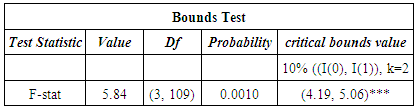
where θ0≡πy.xμ/πyy, θ1≡πy.xγ/ πyy, θ = - πyx.x/ πyy ,  =πy.xC*(L) εt/ πyy (which was derived from πy.x(zt – μ – γt) ) is a zero mean stationary process since the numerator is also a mean zero stationary process [10]. The conditional level relationship between yt and xt gives rise to the conditional unrestricted equilibrium correction model in 1.7. This level relationship was achieved by conducting a joint test of hypothesis8 on the long run coefficients πyy and πyx.x in Table 4. The null hypothesis is rejected if the calculated F-statistic is greater than the asymptotic critical value bounds for case where c0≠0 and c1≠0 as postulated in our conditional unrestricted equilibrium model of 1.7. Table 5 shows the results of the bounds test.For p=3 and k=2, Table 5 shows that the F-value of 5.84 lies outside the upper bounds of the critical bounds value of 5.06 for I(1) on table CI(v) case V on page 301 of [10] when both the intercept and trend are unrestricted indicating that the null hypothesis of no level exchange rate equation is rejected at 10 per cent irrespective of whether the regressors are purely I(0), purely I(1) or mutually cointegrated. Furthermore, t-test on the long-run coefficient of ert-1 is -3.8298 which compared with critical value Table CII(v)9 on pg. 304 of [10] for t-statistic indicates that at 10 per cent level of significance with critical values [-3.13, -3.63], the null hypothesis of no level exchange rate relationship is rejected regardless of the order of integration of the regressors. The result of the bounds test resulted in the estimation of the conditional long-run level relationship model in equation 2.2.
Table 5. Bounds test on Long-run Coefficients in the Unrestricted ECM for testing the existence of level relationships between exchange rate, crude oil prices and inflation rates
 |
| |
|
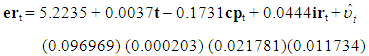 | (2.2) |
Where  is the error correction term with standard error expressed in brackets10. As expected, the level relationship of crude oil price is negative and the inflation rate is positive in the level relationship model. These coefficients are highly statistically significant. This model alongside the conditional unrestricted equilibrium correction model that follows were estimated by adopting the ARDL modelling approach proposed by [15]. The conditional equilibrium correction model associated with the above exchange rate conditional level relationship model is shown in Table 6.
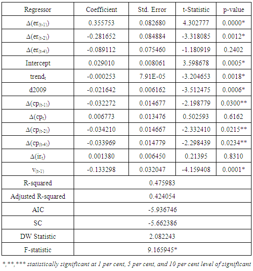
 Table 6. Conditional Unrestricted Equilibrium Correction Model of ARDL (4,4,0) on Exchange rate
 |
| |
|
The results of the conditional unrestricted ECM are similar to the unrestricted ECM in Table 4. All coefficients bear the expected signs and associated standard errors are smaller in the case of the conditional ECM resulting in better estimates of the long-run and short-run coefficients. The  may be referred to as the speed of adjustment to long-run equilibrium (αyx) in the long-run matrix ∏. A highly significant coefficient of -0.13330 (0.03205) implies that about 0.13 per cent of any disequilibrium caused by shocks on crude oil prices and inflation rates is corrected within a month. Alternatively it will take exchange rate about eight months to adjust to any disequilibrium caused by shocks on crude oil prices and inflation rates.
8. Model Stability Check/Diagnosis
The analysis of the autoregressive characteristics polynomial inverse roots shows that the conditional equilibrium model satisfies the stability condition. The LM test statistic value of 0.5919 with p-value of 0.6692 up to lag p =4 signify that the residuals are uncorrelated but not normally distributed which is acceptable since the assumption of εt distributed IN(0,Ω) was relaxed conditionally with mean zero and homoskedastic. This is also shown in the value of the Durbin-Watson statistic which is approximately 2. The inverse root value of 0.0863 with modulus 0.0863 and two complex roots of the characteristic polynomial suggest that our model satisfies the stability condition since no root lie outside the unit circle (figure 4)11. This is further depicted in the impulse response function12 of shock within 1 standard deviation in Figure 3.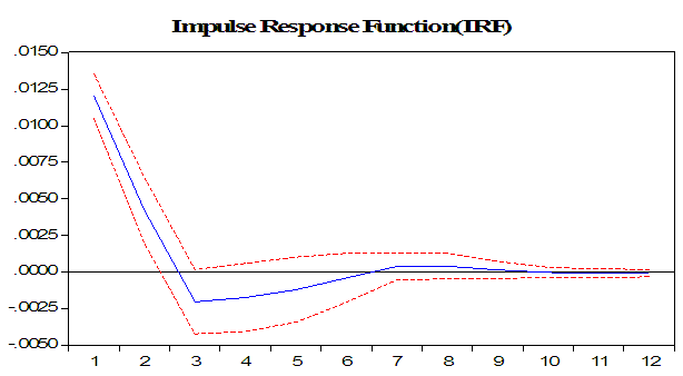 | Figure 3. |
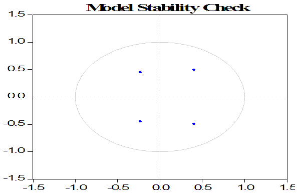 | Figure 4. |
9. Forecast Error Diagnosis and Performance of Model
The evaluation of the historical simulations using scale invariant Theil inequality coefficient shows that a value of 0.0056 is close to zero, unsystematic forecast errors accounted for 99.7963 per cent, the difference between the variance of the forecasts and the actual series accounted for about 0.2005 per cent while bias proportion is 0.0032 per cent indicating a strong association between the actual and forecasted values (Figure 5). Further analysis of the forecast errors which reflected the effects of unsystematic and external shocks on the model revealed that the general elections of 2007 and 2011 had significant effects on the exchange rate movement with former having greater distortions on the forecast residuals than latter. Similarly, the issue of subsidy removal experienced in the first quarter of 2012 resulted in rise of the forecast errors. Also, the mixed effects due to the significant drop in crude oil prices (directly linked with activities of speculators in oil futures)13 between the third quarter of 2008 and first quarter of 2009 was also captured in the forecast errors. These crash in oil prices led to depletion of the country`s foreign reserve by the monetary authority through its exchange rate policy to primarily to achieve macroeconomic stability at the same time expecting a favourable external reserve position and external balance. 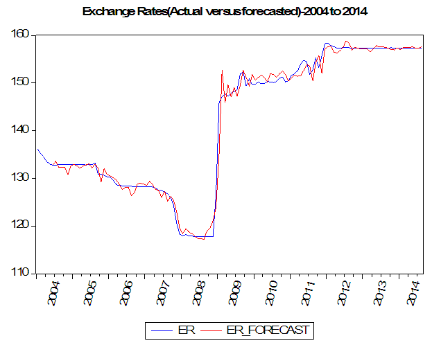 | Figure 5. |
Other unsystematic forces distorting the forecast errors at various points during the period under review include but not limited to reduction in the foreign direct investment (FDI) inflow, faulty trade liberalization policy, and dependence on inefficient foreign exchange market14 and so on. On the global scene, political crisis witnessed in the Middle East and revolutions in countries like Tunisia, Egypt, Libya, Yemen and Syria as well as Iran nuclear crisis, which led to upsurge in the crude oil price at some point, were accounted for in the forecast errors.
10. Conclusions
Crude oil prices and inflation rates are two important determinants of exchange rate stability in Nigeria. The results of ARDL Bounds test discussed in this paper indicated that these macroeconomic variables have significant level relationships with exchange rate in spite of the underlying properties of these series. A marginal coefficient of determination from the global test on the resultant conditional unrestricted equilibrium correction model (ECM) showed that they jointly accounted for a significant portion of the total variability in exchange rate movement in Nigeria. Crude oil prices have an inverse relationship with exchange rate, which is mainly associated with efforts of the monetary authorities to stabilize the local currency through its various exchange rate policies. Inflation rate remained ineffective in the stabilization of exchange rate in the short-run due to issues such as weak export base, excessive demand for foreign exchange, rapidly rising debt burden15, round tripping by authorized dealers amongst other reasons. The exchange rate reacted slowly to shocks on these macroeconomic variables during the period under review. The delay in the reaction of exchange rate particularly to inflationary pressures makes it a weak “shock absorber” during periods of higher inflation. However, the exchange rate model postulated in this paper performed generally well given the results of various diagnostic tests. Furthermore, the findings in this paper substantiate that irrespective of the order of integration of time series, a level relationship can be established using the ARDL Bounds testing approach which eliminates the pre-testing problem associated with alternative methods of cointegration.
Notes
1. Inflation targeting is a monetary policy adopted by the monetary authorities such as Central Bank of Nigeria majorly to achieve full potential production by controlling inflation rate through interest rates [14].2. Yt= γ0 + γ1Yt-1 +.....+ γpYt-p + φ1Xt-1 +.....+ φpXtp + ωt Xt =υ0 + υ1Xt-1 +.....+ υpXt-p + φ1Yt-1 +.....+ ψpYt-p + vt Then, testing H0: φ1 = φ2 = ..... = φp = 0, against HA: 'Not H0', is a test that X does not Granger-cause Y. Similarly, testing H0: φ1 = φ2 = ..... = φp = 0, against HA: 'Not H0', is a test that Y does not Granger-cause X. In each case, a rejection of the null hypothesis implies there is Granger causality[14].3. Quandt-Andrews breakpoint test is a modified version of Chow Test that uses Likelihood Ratio Test. QA breakpoint test follows a non-standard distribution and it automatically computes the usual Chow F-test repeatedly with differing break dates. The Break date with the largest F-statistic is chosen4. The information criteria were calculated for reduced form error correction model.5. Φ(L)(zt – μ – γt) = εt , t = 1,2,3,...............,∞ where the vectors μ, γ are the (k+1)x1 vectors of intercepts and deterministic trend coefficients respectively, Φ(L) is (k+1)x(k+1) polynomial lag operator given as Ӏm - ∑pi=1 ΦiLi6. ∆zt = α0 + α1t + ∏zt-1 + ∑p-1i=1 Γi ∆zt-i + εt where α0 = -∏μ + (Γ+∏ )γ and α1 = -∏ γ are set of constraints on the intercepts and trend coefficient.7. The Nigerian foreign reserve rose by more than 645 per cent from US$8.32 billion in 2004 to US$62.08 billion in September 2008 prior to crash in global crude oil prices associated with speculative trading - CBN statistical database8. H0 = H πyy 0 ∩ H πyx.x 0 vs H1 = H πyy 1 U H πyx.x where, H πyy 0 : πyy = 0 vs H πyy 1 : πyy ≠ 0 and H πyx.x 0 : πyx.x = 0 vs H πyx.x 1 : πyx.x ≠ 0. 9. CII(v) is the Case V for unrestricted intercept and unrestricted trend critical values which computed through probabilistic simulations for testing the null hypothesis ф = 0 using t-statistic in ∆yt = фyt-1 + δ΄xt-1 + α΄wt + ɧt t=1,2,3,....,T [10]10. The standard errors of the coefficients are much smaller than the coefficients signifying the significance of the variables at level.11. Inverse root of autoregressive characteristics polynomial usually should satisfy the condition that all roots must lie within the unit circle indicating stability of the model i.e. │Ӏm - ∑Φizi│≠ 0 for complex z or │z│< 112. See [14] for summary of the procedure on impulse response function13. The crash in crude oil prices by more than 57 per cent led to significant drop in Nigerian foreign reserve by more than 46 per cent from US$62.08 billion in third quarter of 2008 to less than US$33.14 billion in January 2011 – CBN statistical database. 14. Between January 2009 and August 2014, global crude oil price rose by more than 127 per cent but the Nigerian foreign reserve dropped significantly by more than 29 per cent- CBN statistical database.15. The federal government domestic debt burden rose by more than 200 per cent between 2008 and 2013. Similarly, foreign debt burden rose by nearly 97 per cent during the same period. However interest payments continue to move in the same direction as the debt by about 70 per cent between 2008 and 2012 - CBN statistical database. Also, the debt/GDP ratio which measures the relative health of the economy averaged geometrically 35.96 per cent from year 2000 to 2013 representing 4.04 per cent below the fiscal ceiling of 40 per cent.
References
| [1] | Onavwote Victor E., Eriemo O., (2012),“Oil Prices and Real Exchange Rate in Nigeria”, International Journal of Economics and Finance, vol 4, No.6. |
| [2] | Sibanda Kin, Mlambo Courage (2014), “Impact of Oil Prices on the Exchange rate in South Africa”, Journal of Economics, vol 5(2):193-199. |
| [3] | Hassan Suleiman, Mohammed Zahid (2011), “The real Exchange Rate of an oil exporting economy: Empirical evidence from Nigeria” Working paper, Dundee Business School, University of Abertay Dundee, United Kingdom. |
| [4] | Ardian Harri, Lanier Nalley, Darren Hudson (2009), “The Relationship between Oil, Exchange Rates and Commodity Prices”, Journal of Agricultural and Applied Economics, vol.4 (2):501-510. |
| [5] | Selien De Schryder, Gert Peersman (2012), “The US Dollar Exchange Rate and the demand for oil”, CEifo Working Paper Series No. 4126. |
| [6] | Johanna Rickne (2009), “Oil Prices and Real Exchange Rate movements in Oil-Exporting Countries: The Role of Institutions”, Working paper No.810 Research Institute of Industrial Economics. |
| [7] | Usama Al-Mulali, NormeeCheSab (2009), “The Impact of Oil Prices on the Real Exchange Rates of Dirham: A case study of the United Arab Emirates,” Working Paper, MIPRA Paper No. 23493. |
| [8] | Johansen, S. (1988), “Statistical Analysis of Cointegration Vectors”, Journal of Economic Dynamics and Control, 12:231-254. |
| [9] | Sebastian Edwards (2006), “The Relationship between Exchange Rates and Inflation Targeting Revisited”, NBER Working Paper Number 12163. |
| [10] | Pesaran M. Hashem et al (2001), “Bounds Testing Approaches to the Analysis of level relationships”, Journal of Applied Econometrics, 16:289-326. |
| [11] | Said, S.E., Dickey D. (1984), “Testing for Unit Roots in Autoregressive Moving-Average Models with Unknown Order”, Biometrika, 71:599-607. |
| [12] | Dickey D.A., Fuller W.A., (1979), “Distribution of estimators for autoregressive time series with unit roots”, Journal of the American Statistical Association 74:427-431. |
| [13] | Toda, H.Y. and Yamamoto, T. (1995), “Statistical inferences in vector autoregressions with possibly integrated processes”, Journal of Econometrics, 66:225-250. |
| [14] | Aweda Nurudeen O., Akinsanya Taofik, Akingbade Adekunle &Are Stephen O., (2014), “Empirical analysis of the elasticity of real money demand to macroeconomic variables in the United Kingdom with 2008 financial crisis effects”, Journal of Economics and International Finance, 6(8): 190-202. |
| [15] | Pesaran M. H., Shin Y. (1999), An autoregressive distributed lag modelling approach to cointegration analysis, chapter 11in Econometrics and Economic Theory in the 20th century the Ragnar Frisch Centennial symposium, Strom S. (ed.) Cambridge University Press Cambridge. |
| [16] | Engle Robert F., (1984), Handbook of Econometrics, Elsevier Science Publishers BV, 2:776-825. |
| [17] | Johansen, S., J, K., (1990) “Maximum Likelihood Estimation and Inference on Cointegration – With Applications to the Demand for Money”, Oxford Bulletin of Economics and Statistics 51:169–210. |
| [18] | Quandt, Richard E. (1988). The Econometrics of Disequilibrium, Oxford: Blackwell Publishing Co. |
 Abstract
 Reference
 Full-Text PDF
 Full-text HTML