1. Introduction

Epidemiologic rates are often classified in two dimensions. For instance, mortality or cardiovascular disease rates or rates of certain cancers or of performing a surgery are often required to be estimated for both age group and calendar year. These rates are usually higher among the elderly population, and thus for younger age groups they may be unstable as they are likely to be based on small populations at risk. Thus, epidemiologic rates when estimated by age can be unstable. There may also be a systematic time trend in the rates and this may become blurred because of the ‘noise’ or random variation in the estimates. Thus, epidemiologic rates classified in two dimensions may have irregularities in both of them and therefore further use of these rates should require some smoothing in both dimensions. By smoothing we mean a mechanism by which ‘noise’ is reduced from observed data when there is random fluctuation or instability in them.

In this paper, we provide an application and computer programs for a two dimensional method of smoothing rates and counts (eg., event numbers). Epidemiological modelling studies often require smoothing a series of rates in both age and year dimensions before performing actual modelling. Although most existing two-dimensional smoothers are available in the statistical software R, to smooth a series of rates would require additional computer programming by the analyst. To facilitate smoothing a series of rates in two dimensions, we provide programming codes in SAS. It is noteworthy that our aim is to facilitate the practice of two-dimensional smoothing to real life applications. We emphasize on an important property that a smoother should be fairly simple to use [1]. We do not aim to compare the methodological performance of the proposed smoother against existing two dimensional smoothers. This is partly discussed elsewhere [2] and is the scope of another paper. The computer programs we provide are easy to follow and flexible to use. In the next section, we will discuss several epidemiological modelling studies in which a series of rates were required to be smoothed before performing actual modelling. We will use one of these as our case study to demonstrate the usefulness of the smoother.

The two dimensional smoother is a nearest neighbour method based on weighted moving averages. Its estimation rule is straight forward and is computationally simple. It is nonparametric, therefore it avoids making arbitrary assumptions about the shape of the relationships or about their breakpoints. This is of particular importance for settings in which a series of rates or event numbers are required to be smoothed because the shape of the relationships in such situations may not all be the same.

2. Review of Some Modelling Studies Requiring Smoothing of Rates

A number of Markov simulation modelling studies have been conducted for assessing the effectiveness of various CHD risk reduction strategies over time at the population level for different age-sex groups, separately for males and females [2-10]. As part of modelling, these studies required to smooth a series of transition probabilities by both age group and calendar year. Regression models were applied globally rather than locally (which should have been done) in some of these studies [3-10] to smooth all transition probabilities owing to practical convenience. The main problem with this approach is that there will be considerable misspecification bias in fitting certain observed (unsmoothed) age-group-specific and time-specific transition probabilities if their curvatures by age and year dimensions differ greatly. As a result, there would be over- or under- smoothing of these transition probabilities in both dimensions and hence some important features of the data would be lost. This distinction between global and local smoothers is discussed in the next section.

Some Markov modelling studies have inappropriately ignored any instability of the observed transition probabilities by age dimension while smoothing even though both age and year dimensions were considered in the calculation of these probabilities. As a result, they only performed one-dimensional smoothing by smoothing the age-specific transition probabilities in the year dimension. These include the studies discussed above [3-10], a study from insurance in relation to chronic diseases [11] and a study examining the impact of an intervention on coronary heart disease [12].

3. Methods of Smoothing

Methodologically, there are two general approaches to smoothing. One approach is the nonparametric local smoothing which avoids a formal global model and simply performs smoothing based on the local behaviour of the data. By local behavior we mean the behavior of data points required to smooth each data point. Since the data points required to smooth each data point varies, the local behavior of data also varies by the data point to be smoothed. These methods are particularly suitable when there is a series of data to be smoothed. The proposed smoother is suitable for smoothing a series of rates and event numbers.

The other approach to smoothing is to assume a parametric model that is expected to adequately represent the relationships between the variables of interest. Such model based approaches require making arbitrary assumptions about the shape of the relationships or about their breakpoints. The shape of the relationships may not all be the same. This may create practical problems when there are multiple data sets to be smoothed.

When there are several smoothing methods to be compared, the most commonly used approach is the visual comparison of these methods to assess their accuracy in smoothing the data and then choose among them [13]. In this approach, one must plot the observed values and the smoothed values obtained by different methods and examine how the smoothed values capture the trends found in the observed values including any peaks in values and sudden changes.

4. Nearest Neighbour Weighted Moving Average Smoothing Methods

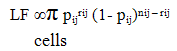
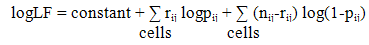
Nearest neighbour smoothing is a group of smoothers which performs smoothing based on the cells which are identified by the analyst to be nearest to the cell which is to be smoothed. The two dimensional nearest neighbour smoother based on weighted moving averages is a type of nonparametric smoother. In the two dimensional nearest neighbour approach, for each cell, a weighted moving average is calculated based on that cell and its nearest neighbouring cells. Weights are assigned to each cell because of the relative importance of the cells with regard to proximity to the central cell. Suppose for each value of the variable X, say x₀, and some fixed value k, the k nearest cells to x₀ are identified and assigned a weight according to their distance from x₀. The smoothed value is equal to the weighted mean of these k neighbours. The smoothness of the resulting curve depends on the value chosen for k and the distribution of weights across the cells. A small value of k will give a rough curve which follows the data points closely, while a large value of k will give a smoother curve.

Since nearest neighbour smoothing outputs a ‘weighted average’ of each cell’s neighbourhood, with the average weighted more towards the value of the central cell, it provides gentler smoothing and preserves the corner points better than a similarly sized equally weighted moving average. By equally weighted moving average we mean a weighted moving average based on equal weights assigned to each cell. This is equivalent to simple or unweighted moving average.

The nearest neighbour smoothers are not greatly influenced (although there is some degree of influence) by any data points which are very far away from the norm or the outliers, since by definition they are locally weighted smoothing techniques using a set of nearest neighbours of each point. A set of weights for which the nearest neighbour smoothing method fits the data best in terms of minimizing the deviance can be considered to be the optimal set of weights for nearest neighbour smoothing.

The theory behind a weighted moving average is that the closer data are more relevant than data further away. When selecting weights for a two-dimensional moving average a logical approach therefore is to give the central cell maximum weight followed by nearest neighbouring cells. However, consideration should be given to whether the same or different weights are to be used around the central cell given that maximum weight has been assigned to the central cell apriori. The simplest approach to choosing weights around the central cell is to give equal weights to these cells. But this may not work well in most situations. The decision to give equal or unequal weights around the central cell should depend on the degree of variability in the data by the two dimensions. For example, while smoothing across age groups and calendar years, if there is more variability by age groups than by calendar years, then more weights should be assigned to cells which belong to the same calendar year but different age groups rather than to cells which belong to the same age group but different calendar years.

One approach to finding such unequal weights around the central cell for nearest neighbour smoothing is to perform a grid search of these weights in two stages. First, the central weight is fixed and the remaining eight weights are generated each taking values starting from 0.05 in a step of 0.05 so that all the nine weights add up to one. Then, the set of weights which fits the data best in terms of reduced -2log (likelihood function) or in abbreviated form -2logLF, are searched. This set of weights are further refined by incrementing each weight by 0.01 within 0.05. Among all such sets of weights the one for which -2logLF is minimum is the optimal or best set of weights.

The mathematical theory for constructing -2logLF is described as follows. Let Pij denote a particular observed transition probability corresponding to ith age group and jth calendar year. If pij denotes the nearest neighbour estimate of Pij, rij denotes the count of events on which this probability is based and nij the population at risk or the denominator of this probability, then the likelihood function assuming that the count of an event (rij) follows a binomial distribution with parameters nij and pij is

(1)

Taking logarithm on both sides we get,

where,

When a binary (event or non-event) experiment is repeated a fixed number of times, say n times, then the count of an event and also the probability of an event both follow binomial distribution. Hence, the use of binomial distribution for constructing the likelihood function above is justifiable. The weighted moving averages defined above are based on the assumption that there is only one lag and one lead in both dimensions (when smoothing the rates) resulting in nine cells in the smoothing bandwidth. If higher lags and leads are to be considered in both dimensions, the bandwidth would increase, for example, 25 cells would be required to smooth the rates if two lags and two leads are considered in both dimensions.

In our case, the term -2logLF based on the set of weights around the central cell which minimizes it is the deviance. Based on large sample theory, it should have an asymptotic chi-squared distribution with error degrees of freedom [14]. The use of chi-squared distribution in this context is to assess the goodness of fit. In our examples for smoothing rates to be shown in the next section, we fix the central cell weight to 0.35. The value of 0.35 is arbitrary. The only criteria is that it should be the maximum of all the weights. Fixing the central cell weight to 0.35 gives a maximum of 0.3 for any of the other weights. Thus, the criteria of assigning maximum weight to the central cell is satisfied. Values higher than 0.35 (but less than 1) could also have been used to fix the central cell weight. However, it should not be too large because of concerns for over-smoothing. A weight of around 0.35 to the central cell is expected to provide gentler smoothing.

5. A Case Study for Smoothing Rates of Cardiac Procedures and Deaths

There are many studies requiring smoothing a series of rates. This is particularly common for modelling studies of health services and chronic diseases involving Markov simulation [2-10]. In this paper, we provide an example of the study by Mannan [2] which predicted from 1990 to 2000 the requirements of coronary artery bypass graft (CABG) and percutaneous coronary intervention (PCI), known together as coronary artery revascularization procedures (CARPs), CHD incidence and deaths in the Western Australian population. In short, the components of the Markov simulation model were initial probabilities of experiencing in a particular year a CARP, CHD admission without a CARP and no CHD admission, all based on hospital admission history, and annual estimates of transition probabilities of moving between these states. The study defined history as any admission to hospital since 1980 for CHD, CABG or PCI. If people experienced more than one coronary artery revascularization procedure (CARP) during this period, we used the most recent of these to define their history. Markov simulation models were developed for every age and sex group separately for males and females. A detailed description of this model is provided elsewhere [2, 15]. The component transition probabilities were classified by age group and calendar year, separately for males and females, therefore there were irregularities in these values in both dimensions. For instance, for younger age groups many of the transition probability estimates were unstable because they were based on small number of observations. Also, there was a systematic trend by calendar year in some of the transition probabilities which became blurred because of the ‘noise’ or random variation in the estimates. Hence a two-dimensional smoother was used to reduce ‘noise’ before performing Markov simulation modelling. The smoothing was done separately for males and females.

This study used a subset of the Western Australian Health Data Linkage System that had electronic records of all hospital admissions and deaths from any form of cardiovascular disease occurring in the period from 1979 to 2001 inclusive. For obtaining the population estimates of Western Australia from 1989 to 2001 the study used Australian Bureau of Statistics (ABS) population data.

6. Smoothing of Transition Probabilities

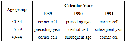
The smoothing examples we provide here are for CABG and coronary death rates classified by calendar years 1990 through 2000 and age groups 35-39 through 75-79. For smoothing the two rates belonging to the 11 calendar years (1990 through 2000) and 9 age groups (35-39 through 75-79), there were 11X9X2 or 198 cells to be smoothed.

For smoothing the transition probabilities, the optimal set of weights are likely to vary by sex and transition probability. For example, if there are 100 transition probabilities to be smoothed belonging to both the sexes, there will be 100X2 or 200 sets of optimal weights.

For each cell corresponding to a particular age group and calendar year, the 9 cells used for smoothing are based on the central cell and its eight nearest neighbouring cells. By central cell we mean the cell to be smoothed. For smoothing every cell, we used the current cell and immediately preceeding and subsequent cells by both the dimensions-age group and calendar year. This results in five cells. While smoothing each cell the rationale for selecting the immediately preceeding and subsequent cells is that the order of the moving average is three. In addition, we used four more cells which are the corner cells. Table 1 clearly shows the cells which are used for smoothing, for example, for the cell belonging to age group 35-39 and calendar year 1990:

Table 1. The Cells Used for Smoothing a Rate Belonging to Age Group 35-39 and Year 1990

Since unweighted or equally weighted moving averages tend to lag the unequally weighted moving averages during large changes in data, we expect that there may also be a similar lag when equal weights are assigned around the central cell with maximum weight assigned to it in comparison to a smooth that also uses maximum weight to the central cell but unequal weights to all cells around it. By lag we mean delay in effect while by lead we mean early occurrence of the effect. For example, if the peak for a rate actually occurred in year 1995 but the ‘noisy’ observed data showed the peak occurring in 1994 then there is a lag of one year in capturing the peak. On the contrary, if the peak occurred in 1996 due to ‘noise’ in the data, then there is a lead of one year in capturing the peak.

To investigate this we use a probability estimate from our study. Figure 1 representing unsmoothed Pr(a CABG|history of CHD) for males by age group shows that for calendar year 1993, these probabilities reach the peak in age group 55-59. This is captured well by nearest neighbour smoothing using unequal weights around the central cell (Figure 2a) while the equal weighting scheme around the central cell shows that this peak occurred in age group 60-64, that is, there is a lag of one age group (Figure 2b).

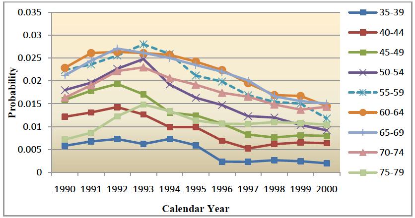
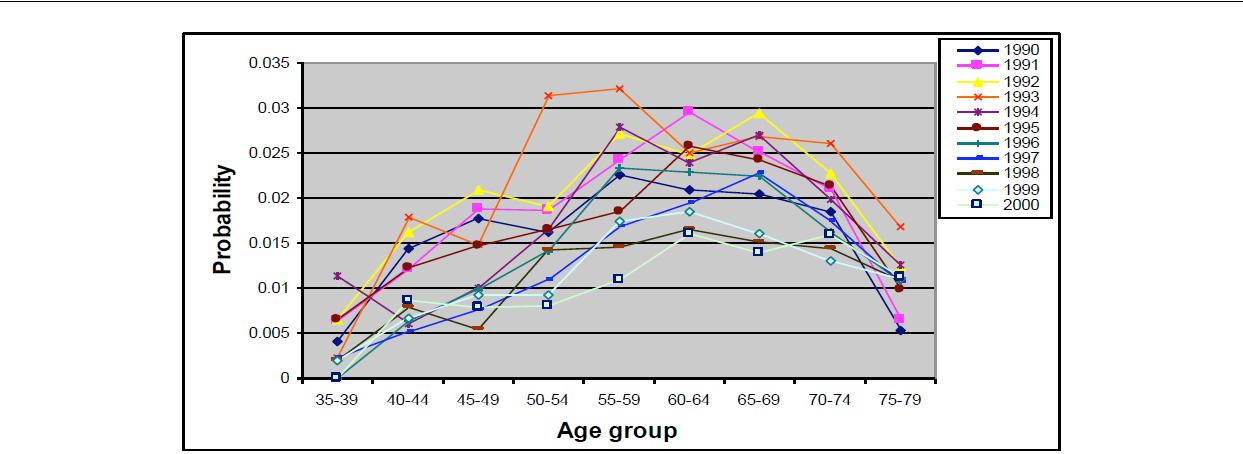Figure 1. Observed estimates of the probability of a CABG given history of CHD, by age group for males

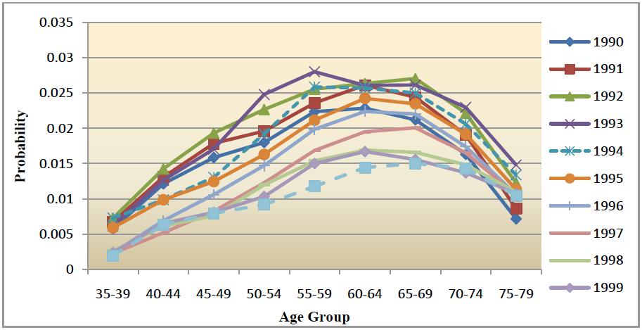Figure 2a. Estimates of probability of a CABG given history of CHD, by age group for males, smoothed by nearest neighbour method using unequal weights around the central cell with its weight fixed at 0.35

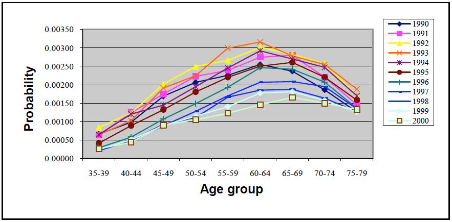Figure 2b. Estimates of probability of a CABG given history of CHD, by age group for males, smoothed by nearest neighbour method using equal weights around the central cell with its weight fixed at 0.35

Using equally weighted moving average to smooth them also sometimes tends to capture earlier the large changes in the values for Pr(a CABG|history of CHD) as compared to the unequally weighted moving average during. For example, Figure 3 shows the observed or unsmoothed estimates of Pr(a CABG|history of CHD) for males by calendar year. Figure 4b shows that using equally weighted moving average around the central cell with its weight fixed at 0.35 captures the large changes in the estimates for Pr(a CABG|history of CHD) earlier compared to the unequally weighted moving average around the central cell with its weight fixed at 0.35, as shown in Figure 4a. The observed probabilities (Figure 3) suddenly increase in 1993 and reach a peak for age group 50-54.

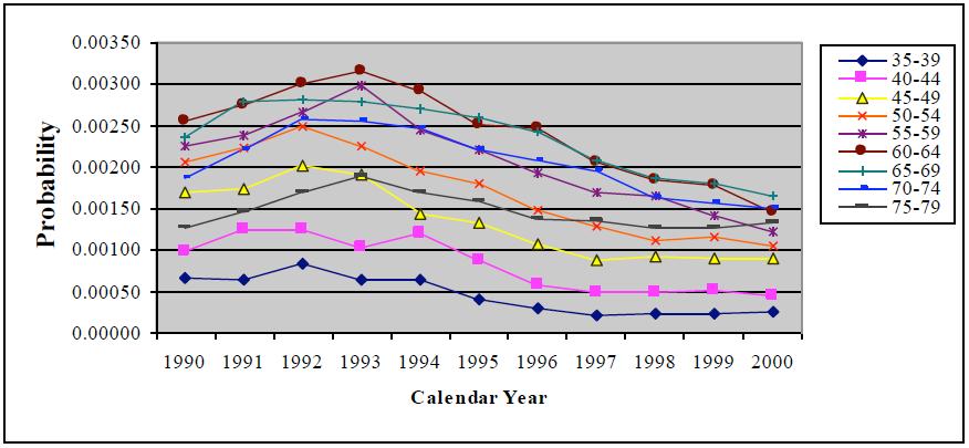
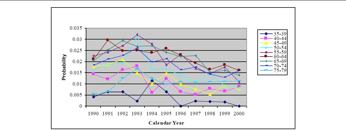Figure 3. Observed estimates of probability of a CABG given history of CHD by calendar year, males

Figure 4a. Estimates of probability of a CABG given history of CHD by calendar year for males, smoothed by nearest neighbour method using unequal weights around the central cell with its weight fixed at 0.35

Figure 4b. Estimates of probability of a CABG given history of CHD by calendar year for males, smoothed by nearest neighbour methodusing equal weights around the central cell with its weight fixed at 0.35

This rapid increase in 1993 is captured well when a nearest neighbour approach with unequal weights has been used to smooth the data while this peak occurs one year earlier in 1992 (Figure 4b) when equal weights are used. Similarly, for age group 60-64 there is a rapid increase in 1994 according to the unsmoothed probabilities shown in Figure 3. This peak is captured well by smoothing using unequal weights around the central cell (Figure 4a) while the weighting scheme which assigns equal weights to all cells around the central cell shows that this peak occurred earlier in 1992 (Figure 4b).

Both the weighting schemes for nearest neighbour smoothing reasonably smooth the observed conditional probabilities as can be seen from the figures. However, the nearest neighbour smooth that allows unequal weights to cells around the central cell captures rapid changes in rates by both calendar year and age group much better than a nearest neighbour smooth that uses equal weights for all cells around the central cell.

7. Sensitivity Analysis

A sensitivity analysis was performed using some selected transition probabilities to evaluate the calibration of nearest neighbour smoothing using unequal weights around the central cell against the same smoother which used equal weights around the central cell. The results are summarised in Table 2. The results demonstrated that calibration was better in terms of reduced deviance when our smoother was used. As expected, the results of this sensitivity analysis suggest that the fit of the transition probabilities improve in terms of reduced deviance with increase in the weight given to the central cell.

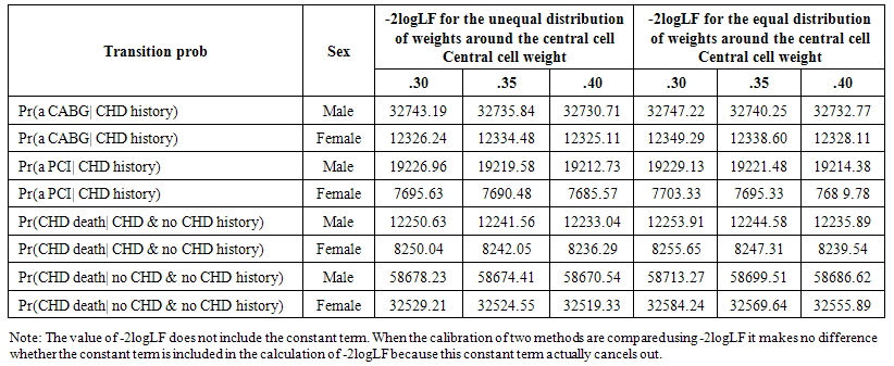Table 2. Deviance for the Nearest Neighbour Smoother with Unequal and Equal Distribution of Weights Around the Central Cell Based on Some Selected Transition Probabilities

8. Computer Codes for the Proposed Smoother

Appendices 1 through 7 provide SAS programming codes including Macros for smoothing the two rates, namely, Pr(a CABG|CHD history), for males and Pr(CHD death|CHD history), for females. It is included in a web site. The example is provided for the central cell weight fixed at 0.35. With this condition the maximum weight for any other cell can be 0.30 so that all weights add up to 1. For other central cell weights the SAS codes can be modified accordingly. However, the codes are flexible to smooth more than two rates by stacking these rates in a sequence and by increasing the number of matrices to more than two as required. In our codes x[11, 13, 2] is used to input the observed data and p[9, 11, 2] is used to output the weighted moving averages. The last dimension of these arrays, that is 2, indicates the number of rates to be smoothed. For smoothing more than two rates, this number should be altered accordingly. The other changes needed to apply the given codes to nearest neighbour smoothing of 3 or more sets of probability estimates or rates are as follows.

The number of elements defined under the array (for the smoothed estimates) p[ ] should also be increased to 297, 396 and so on at the increment of 99 each time a new set of observed probabilities with 99 values required to be smoothed are appended to the dataset. Similarly, the dimensions for the arrays r[ ] and n[ ] should be increased to 297, 396 and so on at the increment of 99.

9. Available Programs for Other Two Dimensional Methods for Smoothing Rates

To our knowledge, there are several computer packages and built-in functions in R implementing two dimensional smoothers which could be used for smoothing a series of rates in two dimensions. The R package ‘Smoothie’ uses Fast Fourier transform which is useful for smoothing a series of rates classified in two dimensions. Multivariate adaptive regression spline (MARS) is available in R through several packages (eg., earth, mda, polspline) and the more recently developed Fast adaptive penalized spline [16] which is computationally faster than MARS is available in the R package ‘AdaptFit’. Both these smoothers are fairly complex mathematically but are accurate and flexible in capturing varying shaped curvatures and are therefore suitable for smoothing a series of rates classified in two dimensions. The well-known Loess smoother, although originally developed for one dimensional smoothing, can perform two dimensional smoothing and has been built into R and all major statistical packages. However, for smoothing a series of rates in two dimensions using either Loess or MARS or Fast adaptive penalized spline or Fast Fourier transform, would require some additional programming using R or any other statistical package in which the smoother has been implemented.

There are a number of smoothers which are suitable for smoothing a series of rates in two dimensions but their use is restricted because of their unavailability in statistical softwares. These include, among others, head banging [17] and the more recently developed ASMOOTH [18] which uses adaptive kernel smoother based on Poisson error. The latter is more suitable for smoothing of small counts and rates/risks.

The R package ‘MortSmooth’ uses P-spline for two dimensional smoothing. This method has fixed knots and is non-adaptive to the varying curvature of the data and is cumbersome to smooth a series of rates in two dimensions. Although Kriging [19] has been implemented in R and can perform two dimensional smoothing and has an adaptive version, its use is restricted to smoothing geospatial data.

10. Findings

Using some selected transition probabilities we showed that our smoother eliminates any lag in changes in data, captures the large changes and time trends well and also reduces overall noise. We also performed a sensitivity analysis using several selected transition probabilities to evaluate the calibration of our smoother against a similar smoother which used equal weights around the central cell. The results demonstrated that calibration was better in terms of reduced deviance when our smoother was used. The calibration of the data improved in terms of reduced deviance with increase in the weight given to the central cell demonstrating that the central cell weight operates as an indicator of the degree of smoothing, with the degree of smoothing increasing with the assigned central cell weight. Thus, it is easy to control the degree of smoothing for our smoother.

For our two example datasets, we noted that when the PACF plot was performed for the year-specific rates against their lags, it showed a significant spike only at lag 1 indicating that all the higher-order autocorrelations were effectively explained by the lag-1 autocorrelation (results not shown). The partial autocorrelation function (PACF) plot [20] plots the partial correlation coefficients between the time series and their lags, and is typically the best approach to determine the order of moving averages. Thus, we used a width of 3 cells in both dimensions with one lag and one lead around the central cell in each dimension resulting in nine point weighted moving averages which included the central cell and all cells surrounding the central cell belonging to the immediately preceding and subsequent age group or calendar year, respectively.

We noted that a number of epidemiological modelling studies [3-12] inappropriately used global smoothers to smooth rates or risks which were classified in two dimensions. Also, they ignored any instability of rates/risks by age and simply considered instability by year even though these rates/risks were classified by both age and year dimensions. Our smoother is an appropriate and convenient approach in such contexts as we have provided SAS codes in this paper (see Appendices 1-7).

11. Discussion

In this paper we have demonstrated the usefulness of a two-dimensional nearest neighbour smoother based on weighted moving averages by providing its associated computer programs in the form of SAS macros. The smoother generally requires no iteration for estimation and involves no computational difficulties. It is a type of box kernel smoother which is a weighted moving average with a fixed width but a variable bin. The difference between our smoother and a typical box kernel smoother lies in the method for estimating the weights. To estimate weights the proposed smoother minimizes the local deviance based on the local likelihood while for estimating weights the box kernel uses the bandwidth and the distance between each cell within the bandwidth and the central cell to be smoothed. The SAS programming examples being provided were for smoothing successively two rates-one for a CABG procedure and another for CHD death, both conditional on having a history of CHD. However, the computer programs can be adapted to smooth successively more than two rates or event counts as needed.

It may be noted that there is a trade-off between variance and bias when more points are used for smoothing because this reduces variance in the data but increases bias. So, there is always a risk of over-smoothing if too many points are used for smoothing. Hence, using simulated data we showed in another study [21] that our smoother avoids over-smoothing and outperforms in terms of reduced deviance a similar nearest neighbour smoother which uses equal weights around the central cell. In practical applications it is preferable to use a smoother that is simple and appropriately reduces lag and yet smoothes enough to reduce noise. Our smoother achieves these objectives.

In our examples, the central cell weight was fixed at 0.35. In most situations, a central cell weight of around 0.35 can perform gentler smoothing. However, if there is still some under- or over-smoothing in our smoothed transition probabilities, it cannot be quantified from our analysis because we used real datasets and hence do not know the distribution of noise in the observed transition probabilities. As has been discussed above, using simulated data we have examined this in another study [21].

The weights for our smoother were selected as such they minimized the error or deviance. This deviance was estimated by a local binomial likelihood which can be approximated well by a local Poisson or Negative Binomial likelihood if there are many zero values for a rate or event count in both dimensions. SAS codes for the latter are available in request from the author.

For finding the optimal weights, we used a two-step procedure. First, after fixing the central cell weight to 0.35, the remaining eight set of weights were selected at multiples of 0.05 with a maximum of 0.30 for any of these cells so that all weights added up to one. The set of weights which minimized -2logLF were selected. In the second step, these weights were incremented by 0.01 so that the final set of weights became more accurate. For even greater accuracy, the weights selected in the second step can be further refined by incrementing them by 0.001 and continuing this process until there is minimal improvement in -2LogLF. This would then become an iterative process for selecting the optimal weights for smoothing. As an alternative approach to finding the optimal weights, we can perform non-linear programming using SAS PROC NLP or maximum likelihood estimation using SAS PROC NLIN. SAS codes using these approaches are available from the author upon request. However, we did not observe any noticeable difference in the results for these approaches compared with our approach.

For practical purposes using a longer width for smoothing would require more data. When there are many levels in both dimensions similar to the examples provided in this paper, such high amount of data may not always be available for all the variables to be smoothed. Thus, using a longer width for smoothing may not always be practical from the requirement of data availability. The well-known Loess smoother can also perform two-dimensional smoothing but requires fairly large, densely sampled data sets in order to produce good models. This is because it needs good empirical information on the local structure of the process in order to perform the local fitting. Since our smoother is based on a weighted moving average rather than local fitting in a small neighbourhood for each subset of a dataset to be smoothed, it would generally require less data than Loess for smoothing. The data requirement for a conventional adaptive box kernel is similar to our smoother. There is a package in R for this smoother. However, for smoothing a series of rates one has to write computer programs in R with the use of this package.

One limitation of our approach is that a local weighted moving average may not always approximate the underlying relationship well enough. For smoothing irregularities like sudden shocks and large bumps, it will not perform well. In such situations, weighted moving medians are expected to perform better. Our smoother is also not completely resistant to outliers. In case of our examples, we did not observe outliers. In situations having outliers when the observed rate is classified in two dimensions, the weighted moving median or robust Loess [22] is more accurate to smooth rates. While the weighted moving median is quite robust to outliers too many outliers even can overcome the robust Loess. The SAS codes for weighted moving median are available from the author.

Finally, in our SAS programming example, we used a fixed dimension for the data matrix based on observed transition probabilities. The example we used was for 11 by 13 dimension for the two transition probabilities we smoothed. However, this dimension does not necessarily have to be the same for all the data (rates or counts) to be smoothed. The SAS codes can be modified to incorporate these changes.

12. Conclusions

In this paper we have demonstrated an application of a nearest neighbour smoother from chronic disease and health services research, for smoothing rates in two dimensions. This method provides a simple alternative to a number of two dimensional smoothers available in the literature which can be used for smoothing rates. We have provided SAS programs including macros for smoothing two rates successively which can be adapted to smooth more than two rates or event numbers if required. The smoother is localized and nonparametric and is flexible for smoothing varying degrees of curvatures. It can capture important changes in data quite well and outperforms a similar nearest neighbour smoother based on equally weighted moving averages around the central cell. A limited comparison of our smoother with some existing smoothers was performed in another study [2]. A detailed comparison of our smoother with some existing adaptive two dimensional smoothers would be the scope of another study.

Supplemental Materials

The supplemental materials can be downloaded from the journal website along with the article.

Appendix

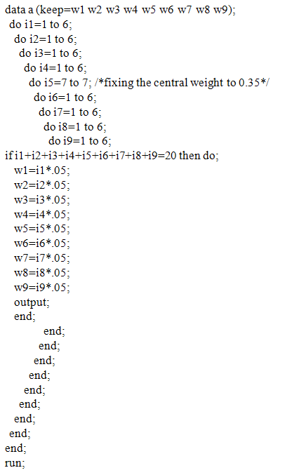
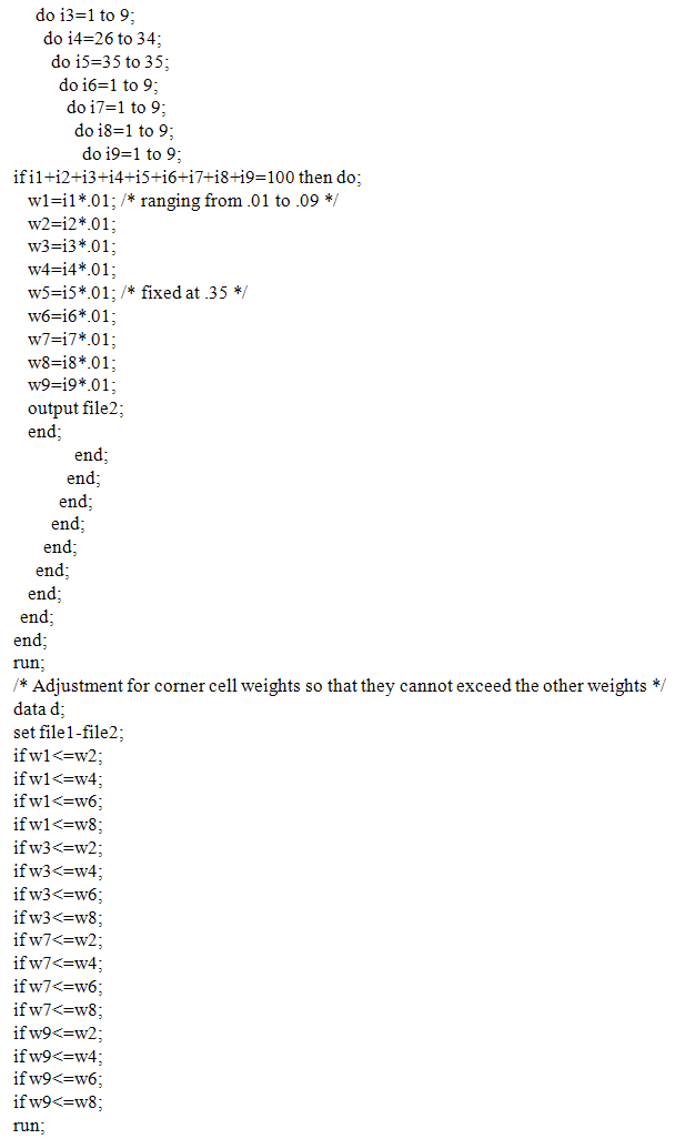
Appendix 1: SAS Codes for Finding All Possible Combinations of Weights around the Central Cell with Its Weight Fixed at .35

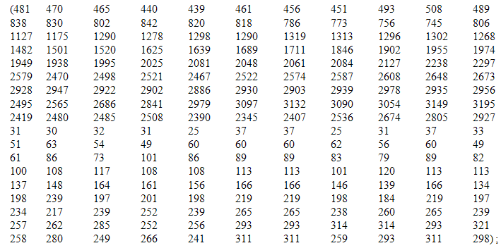
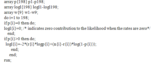
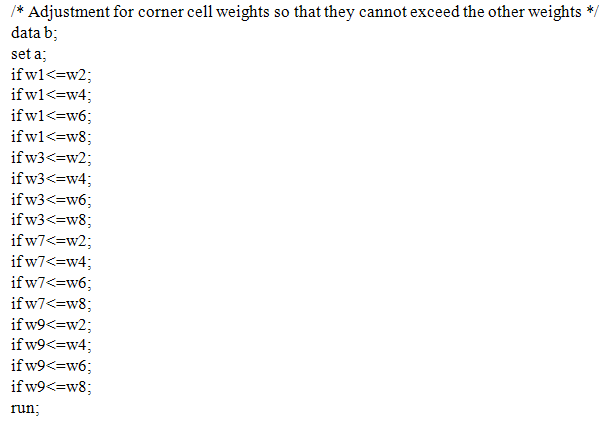Appendix 2: SAS Codes for Finding -2logLF for the Two Rates Using Different Weight Sets Defined in Appendix 1

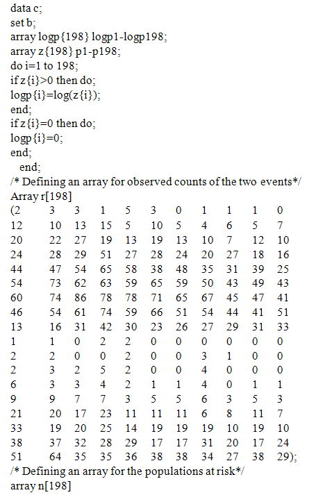
Appendix 3: A SAS Macro for Finding the Deviance and the Initial Optimal Weight Sets for Smoothing the Two Rates

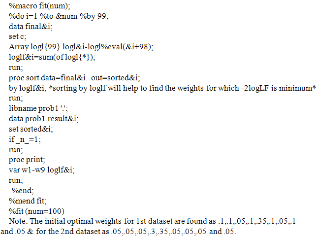Appendix 4: SAS Codes for Refining the Initial Optimal Weights by an Increment of .01 Given the Initial Optimal Weights for Smoothing the First Rate are .10,.05,.05,. 15, .35,.10,.05,.05,.10 & for the Second Rate are .05,.05,.05,.3,.35,.05,.05,.05 and .05

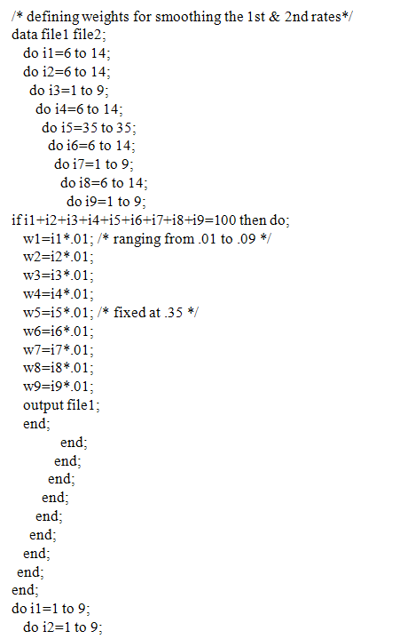
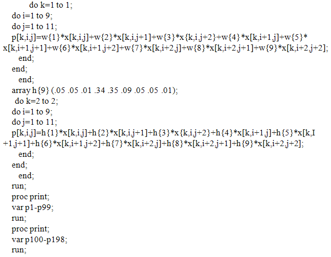
Appendix 5: SAS Codes for Finding -2logLF for the Two Rates Using Different Weight Sets Defined in Appendix 3

These codes are not shown here as they are the same for Appendix 2 except that the SAS file to be read is d and the output SAS dataset saved is e.

Appendix 6: A SAS Macro for Finding the Deviance and the Final Optimal Weight Sets for Smoothing the Two Rates

These codes are not shown here as they are identical to Appendix 3 except that the SAS file to be read is e.

Note: After running this macro the optimal weights for the first rate are found as .09,.09,.01,.14,.35,.13,.01,.09,.09 & for the second rate as 05,.05,.01,.34,.35,.09,.05,.05 and .01.

Appendix 7: SAS Codes for Estimating the Smoothed Values of the Rates

data final;

/* We define an array for entering the data for two conditional probabilities, the examples given here are for Pr(CABG|CHD history, males) and Pr(CHD death|CHD history, females), both for years 1989 through 2001, and age groups 30-34 through 80-84*/

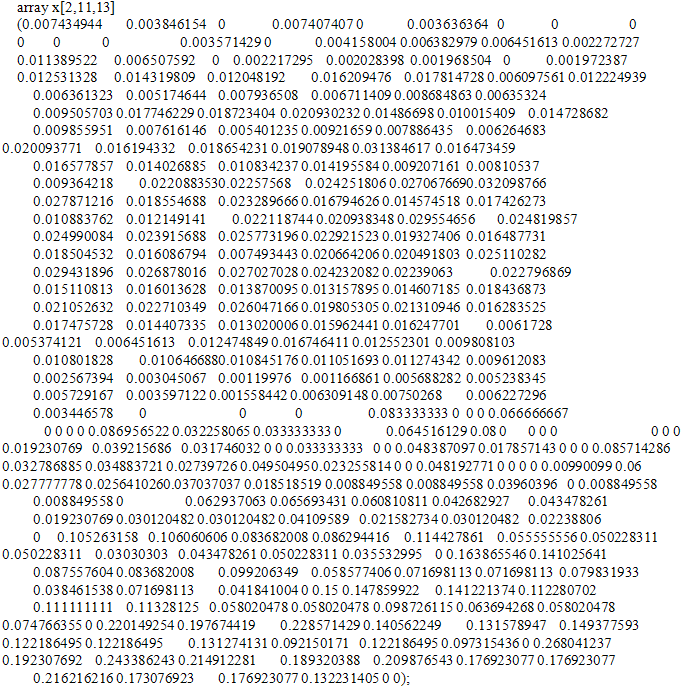array p[2,9,11] p1-p198;

array w{9} (.09 .09 .01 .14 .35 .13 .01 .09 .09);

/* Calculate the nearest neighbour weighted moving averages for the two rates respectively for age group 35-39 and year 1990, age group 35-39 and year 1991, and so on until age group 75-79 and year 2000.*/