1. Introduction

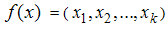
Experiments are performed by researchers in every fields of inquiry so as to study and model the effects of several design variables on the responses of interest. The foundation for response surface methodology (RSM) was laid by [5]. Response surface methodology consists of statistical and mathematical techniques for empirical model building and model exploitation. It seeks to relate a response or output variable to the levels of a number of predictors or input variables that affect it. The form of such a relationship is usually unknown, but can be approximated by a low-order polynomial such as the second-order response surface model

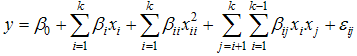(1)

Where y is the measured response, β’s are parameter coefficients; x_i’s are the input variables and is an error term. Most second order designs especially the Central composite design utilize this stated model. However, the Central Composite Design (CCD) is the most popular of the many classes of RSM. It is widely used for estimating second order response surfaces. Since introduced by [5], the CCD has been studied and used by many researchers. [24], suggested several criteria which can be used in the selection of design. [22] studied the duplication of the cube and star points of the CCDs (RCCD and OCCD) for factors k = 2, 3… 8. The results showed that duplicating the star portion has better potential for improved precision of prediction than duplicating the cube portion. [23], evaluated optimum composite design under in different region of interest. [25], suggested optimal CCDs under several design criteria. [19], evaluated and compared three CCDs -Central Composite Circumscribed design (CCC),Central Composite Inscribed design (CCI) and Central Composite Face Centered design (CCF) from the view of region of interest and robustness with simulation. [7] did a comparison of prediction variance performance of some central composite designs in a spherical region. The designs considered were central composite design (CCD), small composite design (SCD) and minimum resolution v design (Min Res). [8] used the D-optimality criterion to compare partially replicated cube and star portions of the rotatable and orthogonal CCD. Their results indicate that replicating the cube portion enhances the D-optimal performance of the CCD more than replicating the star portion. [21] did a graphical evaluation of prediction capabilities of partially replicated orthogonal CCD. They pointed out that replicating the star portions of the CCD considerably reduces the prediction variance, thereby improving the G-efficiency in the spherical region.

In this paper, five varieties of central composite design (SCCD, RCCD, OCCD, Slope-R and FCC) will be evaluated and compared using the D, G, A and IV optimality criteria for factors k = 3, 4, 5 and 6. For factors k = 3 and 4 considered in this paper, full factorial portion of the CCDs are employed while half replicate of the factorial portion of the CCDs are employed for factors k = 5 and 6. The performance of these designs will be considered when the axial portions are replicated and center points increased one and three times. However, because a design may be superior by one optimality criterion but may perform poorly when evaluated by another optimality criterion, fraction of design space (FDS) plot will also be used to evaluate the prediction capabilities of these designs. The findings of this study have wide applications in industrial processes especially in the chemical industry. For example, data resulting from an investigation into the effect of three variables, reaction temperature (x₁), reactant concentration (x₂) and reaction pressure (x₃) on the percentage conversion of a chemical process (y). Other areas of data applications of CCDs can be seen in [14].

1.1. Central Composite Design

The central composite design (CCD) is a design widely used for estimating second order response surfaces. It is perhaps the most popular class of second order designs. Since introduced by [5], the CCD has been studied and used by many researchers. It consists of 2^k full or 2^k-1 half replicate (k is the number of independent variables) factorial points (±1,±1, …,±1); 2k axial or star points of the form (±α, 0,…, 0), (0,±α,… , 0),and a center point (0,0,…,0). In this work, full factorial points will be used for factors k = 3 and 4 while half replicate factorial points will be for factors k = 5 and 6. The axial points will be replicated one and two times while the center points will be replicated one and three times. The center points provide information about the existence of curvature in the the addition of axial points allow for efficient estimation of the pure quadratic terms. The choice of the number of center runs provides flexibility to get a better estimate of the pure error and better power for test. Moreover, the choice of the number of center runs affects the distribution of the scaled prediction variance. The factorial points allow estimation of the first-order and interaction terms. Let N denote the total number of experimental runs in the CCD, 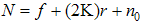. Here f is the number of factorial points, 2k is the axial points which is replicated r times and n₀ the center points. The choice of axial distance α is based on the region of interest. Choosing the appropriate values of α specifies the type of CCD. To be able to make use of these varieties, the researcher must first understand the differences between these varieties in terms of the experimental region of interest and region operability, [17]. The region of operability for the CCDs considered in this paper is the spherical region except FCC which is employed if the primary region of interest is cuboidal.

1.1.1. Spherical Central Composite Design (SCCD)

Setting α =, makes the CCD a spherical CCD. In spherical CCDs, all design points occur on the same geometric sphere. Spherical CCDs are not exactly rotatable, but they are near-rotatable.

1.1.2. Rotatable Central Composite Designs (RCCD)

In RSM, rotatability is considered as one of the desired properties of the second order designs. The concept of rotatability was first introduced by [4], in the rotatable design the variance of the predicted response ŷ(x) depends on the location of the point that is, it is a function only of distance from the point to the center of the design. By definition, a design is rotatable if is constant at all the points that are equidistant from the center of the design. Setting makes CCD rotatable. Where ƒ is the factorial points

1.1.3. Orthogonal Central Composite Design (OCCD)

A 2^k factorial design and the fractional factorial 2^k-1 design in which the main effects are not aliased with other main effects are orthogonal designs. Consider a second order model with pure quadratic terms corrected for their means.

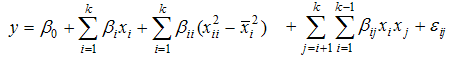(2)

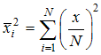Where . Let denote the least square estimators of respectively. In the CCD, all the covariances between estimated regression coefficient except are zero. But if the inverse of the information matrix is a diagonal matrix, then also becomes zero. This property is called orthogonality. The condition for making a CCD orthogonal is by Setting 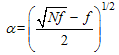see [13]. Where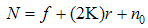, . The orthogonal CCD provides ease in computations and uncorrelated estimates of the response model coefficients.

1.1.4. Slope Rotatable Central Composite Design (Slope-R)

Suppose that estimation of the first derivative of η(x) with respect to each of the independent variables. For the second order model,

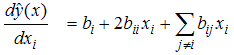(3)

The variance of this derivative is a function of the point x at which the derivative is estimated and also a function of the design through the relationship

(4)

[20] proposed an analog of the Box-Hunter rotatability criterion, which requires that the variance of be constant on circles (k=2), spheres (k=3), or hyperspheres (k≥4) centered at the design origin. Estimates of the derivative over axial directions would then be equally reliable for all points x equidistant from the design origin. They referred to this property as slope rotatability, and showed that the condition for a CCD to be a slope –rotatable is as follows

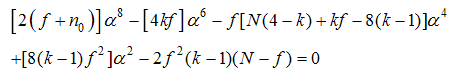(5)

From (5), the values of for slope-rotatable central composite design are evaluated. See [20].

1.1.5. Face Center Cube (FCC)

Setting α = 1 makes the CCD, a Face-centered CCD and also a three level design. The axial and the factorial points of face-centre CCD fall onto the surface of the cube. The face-centered cube CCD does not require center points because of the existence of ()^-1. But center points are included for testing for lack of fit.

1.2. Optimality Criteria

Optimal designs are experimental designs that are generated based on a particular optimality criterion and are generally optimal only for a specific statistical model. Optimal design methods use a single criterion in order to construct designs for RSM; this is especially relevant when fitting second order models. [12] detailed the theory behind optimum designs.

An optimality criterion is a criterion which summarizes how good a design is, and it is maximized or minimized by an optimal design. Design optimality is often called the alphabetical optimality criteria because they are named by some of the letters of the alphabet.

1.2.1. D-optimality

When considered historically, D-optimality by [18] was the first alphabetical optimality criterion developed. It is the most well studied problem which is seen in the literature by [12], [15], [1], [16] and [10]. It is also still among the most popular because of its simple computation, and many available algorithms.The D-optimality focuses on the estimation of model parameters through good attributes of the moment matrix which is defined as , where is the information matrix and N, the total number of runs, is used as a penalty for the larger design. D-optimality seeks to maximize the determinant of the information matrix or equivalently seeks to minimize the inverse of the information matrix. That is 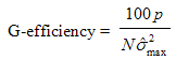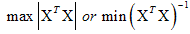. The D-efficiency where p is the number of model parameters.

1.2.2. A-optimality

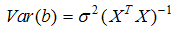
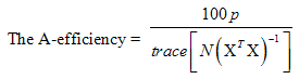
This criterion introduced by [6] seeks to minimize the trace of the inverse of the information matrix (X’X). This criterion results in minimizing the average variance of the estimates of the regression coefficients. Unlike D-optimality, it does not make use of covariance among coefficients.

1.2.3. G-optimality

This criterion is concern with prediction variance. It may be that the aim of the practitioner is to have good prediction at a particular location in the design space. To attain this, [4] defined a variance function, i.e., the scaled prediction variance (SPV). The SPV is defined as

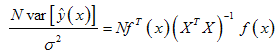(6)

where is the vector of coordinates of point in the region of interest expanded to model form. That is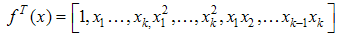, N is the total sample size penalizing the larger designs, X is the design matrix and is the process variance which is assumed to be 1. The SPV provides a measure of the precision of the estimated response at any point in the design space. A G-optimal design is one that minimizes the maximum SPV over the experimental design region. Symbolically, it is written as

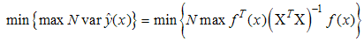(7)

The

1.2.4. IV-optimality

IV-optimality, also called I-optimality and V-optimality in the literature, is based on properties of the scaled prediction variance. Instead of finding maximum prediction variance in the region of interest, it makes use of the average of prediction variance (throughout the region of interest). Hence this gives a measure of the overall distribution of prediction variance. A design is said to be IV-optimal if it minimizes the normalized average integrated prediction variance.

(8)

Where is the prediction variance, R is the region of interest and u is uniform measure on R with total measure 1. This integral was simplified by [3] as

(9)

where S is the moment matrix of region of interest (see also [11])

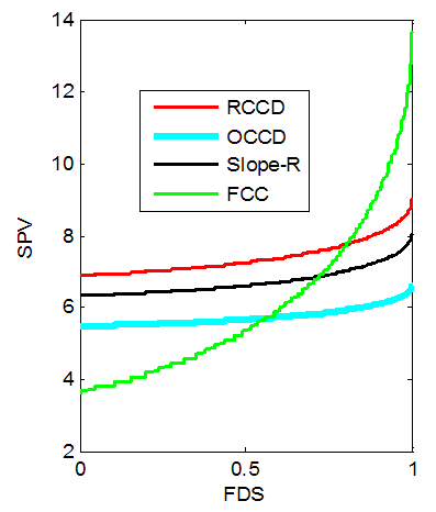
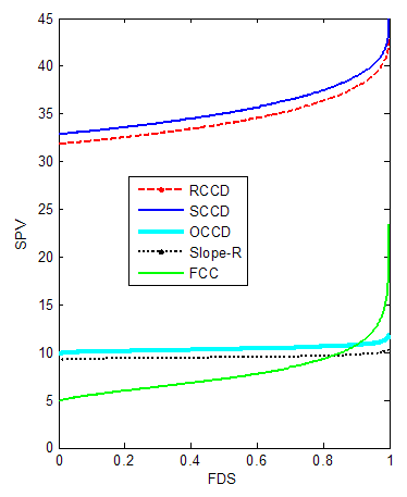
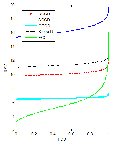
1.3. Fractions of Design Space (FDS) Plots

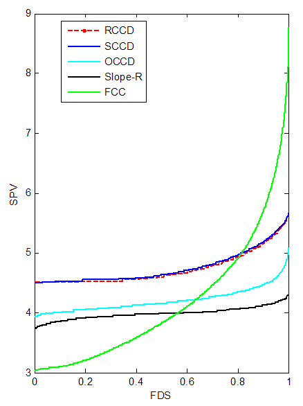
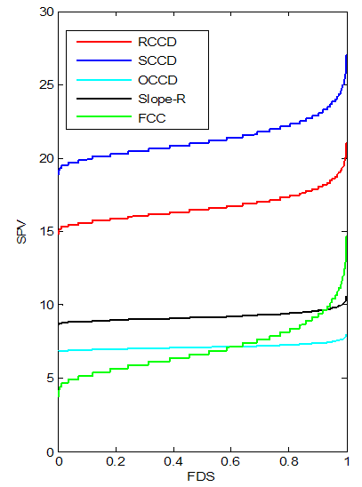
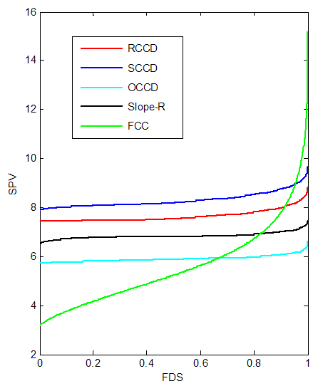
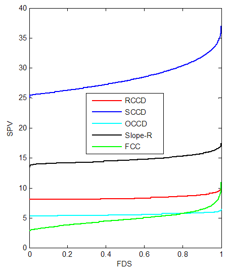
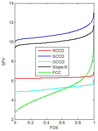
Single-number criteria such as D, A and G-efficiency or IV criterion do not completely reflect the prediction variance characteristics of the design in question. However, a design that is superior by one optimality criterion may perform poorly when evaluated by another optimality criterion. According to [2], by condensing the properties of a design to a single value, much information is lost as regards the design’s potential performance.

FDS plot introduced by [9], as alternative to single-value criteria, overcome this shortfall by displaying the characteristics of the prediction variance throughout the entire design space. The plot also displays characteristics of scaled prediction variance (SPV) throughout a multidimensional region on a single two- dimensional graph, this time with a single curve. The FDS plot shows the fraction of the design space at or below any SPV value. It is constructed by sampling a large number of values, say n, from throughout the design space and obtaining all of the corresponding SPV values which are then ordered and plotted against the quantiles (1/n, 2/n …). The x-axis gives the quantiles of the design space ranging from 0 to 1, while the y-axis shows the SPV values.

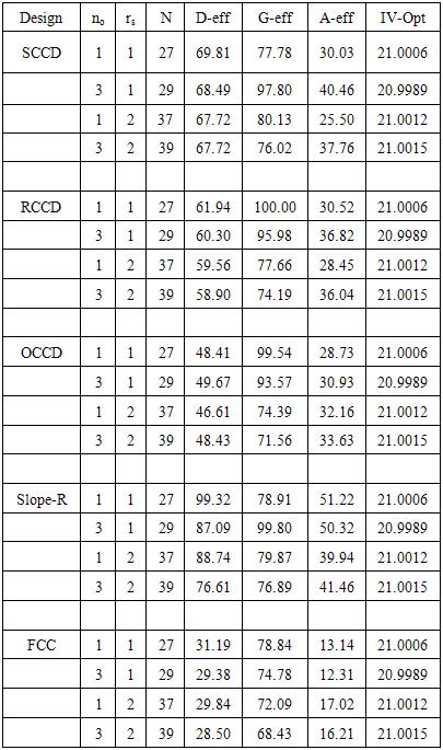
2. Design Comparison

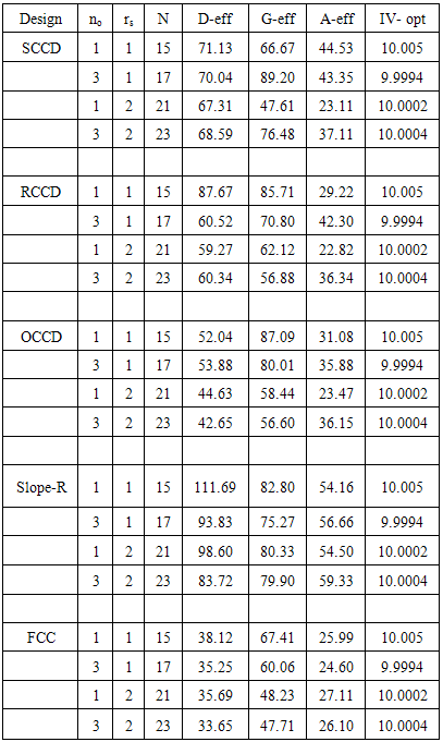
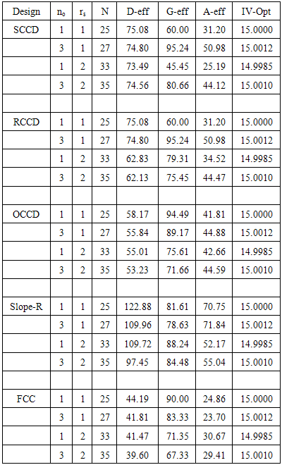
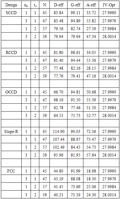
In this section, the D, A, G and IV optimality criteria for the full second order model comparisons of the 5 varieties of CCD (RCCD, SCCD, OCCD, FCC, and Slope-R) for factors k = 3, 4, 5 and 6 are summarized in tables 1, 2, 3 and 4 respectively. For the optimality criteria; larger values imply a better design (on a per point basis). Let r_s indicate the replication of star points of the design and N the number of design runs.

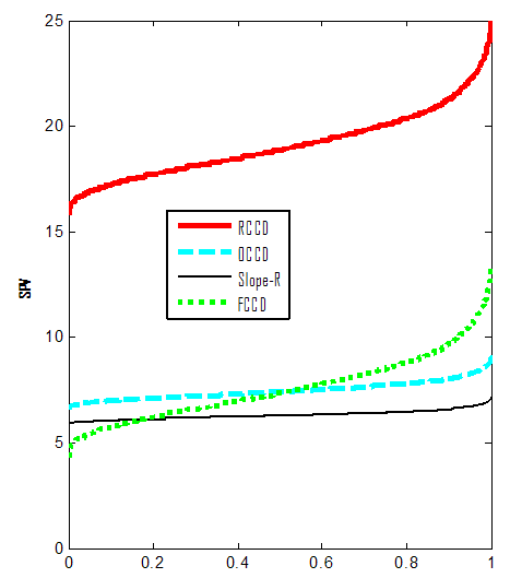
2.1. Three-Factor Design

Table 1 shows that replicating the star points or axial portion (increasing r_s) tends to reduce the D and G-optimality criteria for the CCDs (RCCD, SCCD, Slope-R, OCCD and FCC). In A-optimality criterion, replicating the star points tends to reduce the SCCD, RCCD and OCCD but in vice versa for Slope-R and FCC. Increasing the center points tends to reduce the D- optimality criterion of SCCD, RCCD, FCC and Slope-R except the OCCD. But if the star points are replicated, increasing the center points tend to increase the D-optimality criterion of the CCDs. In G-optimality criterion, increasing the center points tends to reduce the performance of the RCCD, OCCD, FCC, and Slope-R except SCCD.

Table 1. Summary Statistics for Varieties of Central Composite Design for factor k = 3

Increasing the center points also tends to reduce the A-optimality criterion for SCCD and FCC but it is vice versa for RCCD, OCCD and Slope-R portion replicated. In IV-optimality criterion, the CCDs are relatively the same both when the center points and axial portion are increased.

Figure 1 and 2 displays fraction of design space plot for varieties of CCD with 1 and 3 center points respectively.

The design with three center runs (Figure 2) has much smaller prediction variance throughout the design space. In both FDS plot, Slope-R clearly shows a better stable prediction variance over other varieties of CCD. RCCD and SCCD have similar high SPV distribution while FCC has a lower SPV for a small portion of the design space plot but highly unstable.

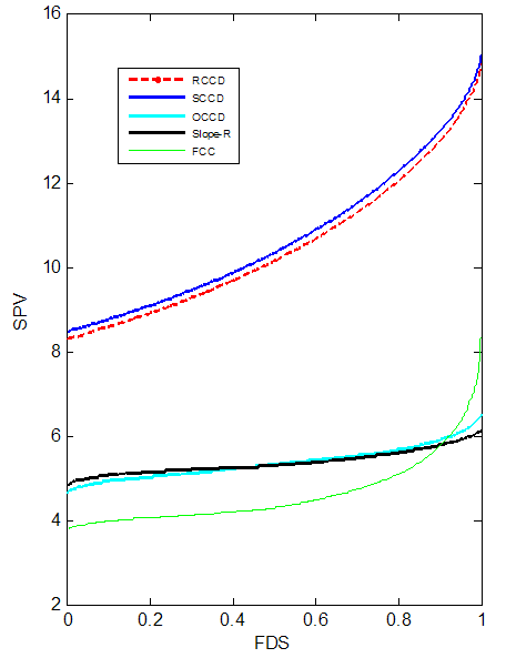Figure 1. FDS Plot of CCD for k =3 with 1 center point

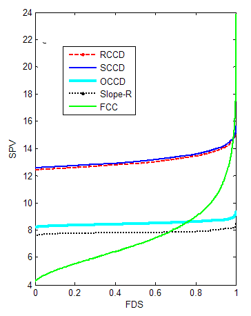
Figure 2. FDS Plot of CCD for k =3 with 3 center points

Figure 3 and Figure 4 also shows FDS plot of varieties of CCD when the axial portion is replicated, with 1 and 3 center points respectively. From the plot, the CCDs maintain relatively a stable and low SPV throughout the design space when the axial portions of the CCDs are replicated with 3 center points. Replicating the axial portions does have no much effect on FCC and OCCD as the still have low SPV with both 1 and 3 center points.

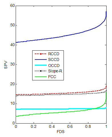
Figure 3. FDS Plot of CCD with replicated axial

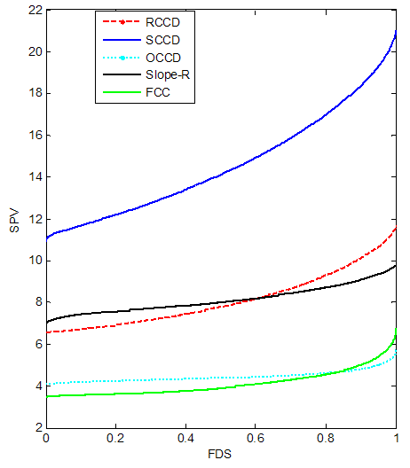
2.2. Four-Factor Design

Table 2 shows that replicating the star points or axial portion (increasing r_s) tends to reduce the D and G- optimality criteria for the CCDs. But for A-optimality criterion, SCCD, RCCD and Slope-R tends to reduce with an increase in axial portion but in vice versa for OCCD and FCC.

Table 2. Summary Statistics for Varieties of Central Composite Designs for factor k = 4

Increasing the center points also tends to reduce the D-optimality criterion for the CCDs. But for G and A-optimality criteria, OCCD, Slope-R and FCC tends reduce with an increase in center points except SCCD and RCCD.

In IV-optimality criterion, the CCDs are relatively the same both when the center points are increased and axial portion replicated.

The FDS plot of figure 5 and figure 6 shows that RCCD has a high SPV over the design space with 1 center point (figure 5) though it reduced with an increase in center points (figure 6), but it is unstable. Slope-R and OCCD relatively maintained a stable SPV over the design space but with an increase in center points, they are slightly unstable. FCC with an increase in center points has a low SPV over a small fraction of design space. When the axial portion is replicated, the FDS plot of figure 8 shows that SCCD has high and unstable scaled prediction variance. RCCD, Slope-R and OCCD maintained relatively a low SPV over the design space.

Figure 5. FDS Plot of CCD for k =4 with 1 center point

Figure 6. FDS Plot of CCD for k = 4 with 3 center points

Figure 7. FDS Plot of CCD with replicated axial portion for k = 4 with 1 center point

Figure 8. FDS Plot of CCD with replicated axial portion for k = 4 with 3 center points

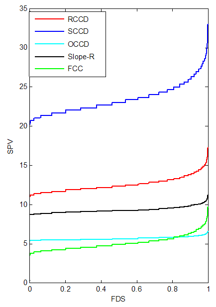
2.3. Five-Factor Design

Table 3 shows that replicating the axial portion tends to reduce the D and G- optimality criteria for the CCDs. Also for A-optimality criterion, replicating the axial portion tends to reduce the performance of RCCD, SCCD and Slope-R but in vice versa with OCCD and FCC.

Table 3. Summary Statistics for Varieties of Central Composite Designs for factor k = 5

Increasing the center points tends to reduce the D-optimality criterion for SCCD, RCCD, FCC and Slope-R. But for OCCD, increasing the center points tends to reduce the D-optimality for the design only when the star points are replicated. Increasing the center points also tends to reduce the G-optimality criterion for RCCD, OCCD and FCC.

Increasing the center points also tends to reduce the G-optimality criterion for RCCD, OCCD and FCC.

But for SCCD and Slope-R, increasing the center points only tends to increase the G-optimality criterion for these designs when the axial portions are replicated. Also increasing the center points tends to increase the A-optimality of SCCD, RCCD and OCCD but in vice versa for Slope-R and FCC. In IV-optimality criterion, the CCDs are relatively the same both when the center points are increased and axial portion replicated.

Figure 9 and Figure 10 displays the FDS plot of the CCDs for k = 5. From the plots, Slope-R and OCCD maintain a relatively stable SPV. But when the center point is increased (Figure 10), SCCD and RCCD had a reduced SPV and also relatively stable. FCC in both FDS plot has low and unstable SPV. Figure 11 and 12 displays the FDS plot of the CCDs when the axial portions are replicated. OCCD, RCCD and Slope-R maintain a stable SPV with 1 center but when the center point is increase (Figure 12), RCCD still maintained a stable and low SPV. With an increase in center points, SCCD, Slope-R and OCCD becomes unstable in spite of relatively having low SPV.

Figure 9. FDS Plot of CCD for k =5 with 1 center point

Figure 10. FDS Plot of CCD for k =5 with 3 center points

Figure 11. FDS Plot of CCD with replicated axial portion for k = 5 with 1 center point

Figure 12. FDS Plot of CCD with replicated axial portion for k = 5 with 3 center points

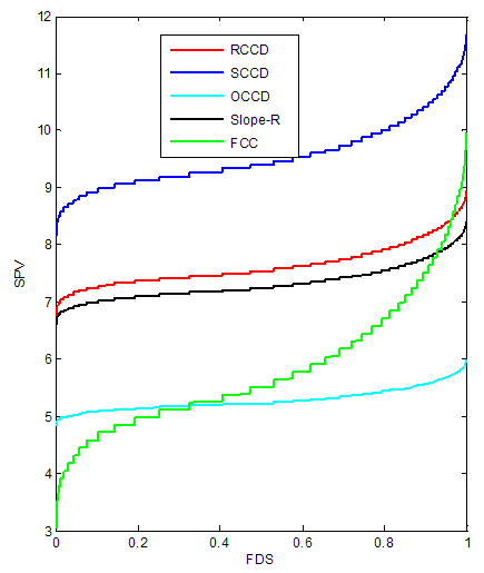
2.4. Six-Factor Design

Table 4 shows that replicating the star points tend to reduce the D and G-optimality criteria for the CCDs. Also replicating the star points tend to reduce the A-optimality criterion for the CCDs except the FCC.

Table 4. Summary Statistics for Varieties of Central Composite Designs for factor k = 6

Increasing the center points tends to reduce the D-optimality criterion for FCC and Slope-R but for SCCD and RCCD, increasing the center points tends to reduce the D-optimality criterion of the design if the star points are not replicated, while increasing the center points tends to increase the D-optimality criterion for the OCCD. Also increasing the center points tends to reduce the G-optimality criterion for the CCDs while also the CCDs tend to increase with increase in center points for A-optimality criterion.

In IV-optimality criterion, the CCDs are relatively the same both when the center points are increased and axial portion replicated.

The Figure 13 and Figure 14 displays the FDS plot of the CCDs for k = 6 with 1 and 3 center points respectively. Figure 13 shows that RCCD and SCCD have high and unstable SPV compared to OCCD and Slope-R that have low and relatively stable SPV. With an increase in center points (figure 14), RCCD and SCCD have a reduced SPV though still high when compared with OCCD and Slope-R. When the axial portion is replicated with 1 center point (Figure 15), the FDS plot shows that OCCD has the most stable SPV compared to RCCD and Slope-R which are competing. SCCD has a high and unstable SPV unlike FCC which has a low and unstable SPV. With an increase in center points (Figure 16), OCCD still maintain the most stable SPV. RCCD performs better than Slope-R with lower SPV. SCCD has a reduced SPV though still high and unstable. FCC covers most of design space but it is still unstable.

Figure 13. FDS Plot of CCD for k =6 with 1 center point

Figure 14. FDS Plot of CCD for k =6 with 3 center points

Figure 15. FDS Plot of CCD with replicated axial portion for k = 6 with 1 center point

Figure 16. FDS Plot of CCD with replicated axial portion for k = 6 with 3 center points

3. Conclusions

Replicating the star points tends to reduce the D and G-optimality criteria for the CCDs. Slope-R performs better than all the designs when D and A –optimality criteria are employed for all the factors considered. OCCD is a better design when G-optimality criterion is employed especially when the star points are not replicated for factors k = 3 and 4. But when the star points are replicated, Slope-R is a better design when G-optimality is employed for factors k = 3 and 4. For factor k = 5, RCCD is a better design when G-optimality is employed and SCCD a better design when G-optimality criterion is employed for factor k = 6. The FDS plots indicates that the CCDs maintain relatively low and stable SPV when the star points are replicated with increased center points. In all the factors considered, the OCCD maintained a better, low and stable SPV when the star points are replicated. The Slope-R has a better low and stable SPV at factor k = 6 when the star points are not replicated.