I. E. Okorie , A. C. Akpanta
Abia State University, Uturu, Nigeria
Correspondence to: I. E. Okorie , Abia State University, Uturu, Nigeria.
| Email: |  |
Copyright © 2015 Scientific & Academic Publishing. All Rights Reserved.
Abstract
Ikeja in Lagos State was one of the major towns in Nigeria that was struck by the 2012 flooding with a devastating economic effect. However, among other major causes of this natural disaster was extreme rainfall. This paper therefore, focuses on extreme value analysis of the Ikeja monthly rainfall (January, 1980 to December, 2012) obtained from the Central Bank of Nigeria (CBN) official website. The set of data shows a very significant periodicity and strong departure from normality. The Generalized Pareto (GP) distribution was adequately fitted to the threshold excesses of the seasonally differenced rainfall data, the shape parameter is not significantly different from zero, and the diagnostic plots did not give any doubt on the goodness of fit of the fitted GP model. The results obtained could serve as a guide to stakeholders in weather and climatic management.
Keywords:
Extreme value analysis, Peak over threshold (POT), Generalized Pareto (GP) distribution, Rainfall, and Ikeja
Cite this paper: I. E. Okorie , A. C. Akpanta , Threshold Excess Analysis of Ikeja Monthly Rainfall in Nigeria, International Journal of Statistics and Applications, Vol. 5 No. 1, 2015, pp. 15-20. doi: 10.5923/j.statistics.20150501.03.
1. Introduction
The 2012 flooding in Nigeria affected 156 local governments where about 7 million people were affected; 2.3 million people fled their homes and 363 people were reported dead and it was further revealed that excessive rainfall was particularly the major cause of the natural disaster that turned into a national disaster [1]. Odunga, et al. [2], in their survey reported that the flooding in Lagos is due to excessive rainfall and has resulted to severe loss of lives and property where monetary loss in bussiness as a result of flooding just from a single storm ranges from $84.75 to $8474.58. Also, Andrew [3] in his work on the analysis of extreme rainfall and flooding stated that the persistent 2 days heavy rain was responsible for the Cumbria 2009 flooding where over 1500 properties were flooded, several bridges collapsed and a traffic directing policeman drowned. Extreme values (minima or maxima) are basically as a result of those events that occur with a very small probability, large in magnitude and usually devastating effect. The study of the stochastic behaviour of the maxima is referred to as the extreme value theory. The inherent behaviour of an independent and identically distributed (iid) extreme values is characterized by one of the following extreme value distributions: Gumbel,  and Weibull, [4].
2. Methodology
2.1. Extreme Value Theory
Here we present the theory which underpins extreme value theory and focus is on the statistical behaviour of the maxima denoted by  . Let
. Let  be iid random variables with common distribution function F thus;
 and let
  be the upper end point of
  we have
  Finite or Infinite maxima (
 ) converges almost surely to the upper endpoint of
  .
.
2.1.1. Extremal Types Theorem
The limit theory is only plausible for possible norming constants  and a non-degenerate distribution function
  such that the distribution function of a normalized
  converges to
  as
as  tends to infinity i.e.
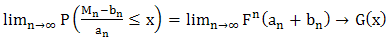 | (1) |
If (1) is true for suitable choices of  ; then we say that
  is the distribution function of
  and
and  is the domain of attraction of
  , written as
  . The extremal type theorem focuses on describing the tail of the distribution. Interestingly, it is an analogy of the central limit theorem which concentrates on describing the centre of the distribution. The limit
  [4], [5], [6], and [7] belongs to one of the following three classes:
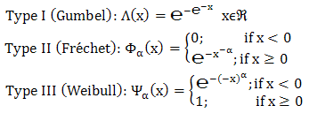 | (2) |
notably, (1) implies that the renormalized maximum  converges in distribution to a variable belonging to one of the three types of extreme value distributions in (2)
2.2. Generalized Extreme Value (GEV) Distribution
The combination of the three distributions in (2) results to a single distribution known as the generalized extreme value (GEV) distribution with distribution function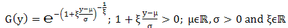 | (3) |
(3) is generalized because the type I, type II and type III in (2) could be obtained when 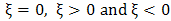 respectively. There are several approaches to modelling extreme values but this work only places emphasis on two methods: block maxima and the peak over threshold1 (POT) approaches.
2.2.1. Method of Block Maxima
The GEV distribution discussed in 2.2 is only a reasonable model for modelling the block maxima. The block maxima approach technically entails the division of the  random variables into non overlapping blocks of equal length and fitting the GEV distribution to the set of maxima resulting from the blocks. The choice of block size is essentially the only sensitive stage in block maxima approach hence, care need to be exercised in choosing an appropriate block size because choosing a too small block size will result to bias estimation and extrapolation, while large blocks provides few block maxima leading to inflation of the estimator variance [8]. Hence, reasonable block size provides a happy compromise between bias and variance. For example rainfall is seasonal and this renders a block of size 3 or 4 ineffective because the second or third block in a year is likely to have the highest maximum rainfall across the period of investigation and inference based on this would be inaccurate and misleading because of the violation of the prior assumption of
  for
for  in 2.1. Since we are confronted with a monthly data taking a block of length one year (annual blocks) in this case would satisfy the assumption that the individual block maxima have a common distribution. Since
  is assumed to be
  it immediately follows that a realization of block maxima denoted by
  is further assumed to follow a GEV distribution and could adequately be modelled by the GEV distribution.
2.3. Pot Method and Generalized Pareto (GP) Distribution
Imagine the situation where not only one observation emerged as the maximum in a particular block but many, resulting to variation in the block maxima; in this scenario it is likely to miss out the relevant information about the upper tail of the inherent probability distribution since the number of extreme values will differ from block to block. The above limitation of the block maxima method quickly lends motivation to a more modern approach known as the POT method for modelling all large observations exceeding a certain threshold u.Suppose there exist a distribution  such that its extreme values can be renormalized in such a way that the renormalized extreme values converges asymptotically to the GEV distribution where a threshold
  could be chosen such that observations above it (exceedances) could appropriately be modelled by the generalized Pareto (GP) distribution with distribution function
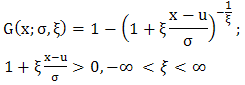 | (4) |
Where,  and
and  are the only two parameters of the GPD corresponding to the scale and shape parameters, respectively.
  is the threshold value 'not a parameter' the GP distribution is generalized because it assumes different distributions in the same sense as the GEV when
  in (4) takes the following values:a.
  , implies a medium size tailed distribution with finite or infinite right end point (unbounded). E.g.: the Normal distribution, the Exponential distribution, the Gamma distribution, the Log-normal distribution and the Gumbel distribution. In this special case all the moments exist.b.
  , implies a light tailed distribution with a short decay and a finite right end point (bounded). E.g.: the Weibull distribution, the Uniform distribution and the Beta distribution.c.
  , implies a heavy tailed distribution with an infinite right end point (unbounded) which decays at a polynomial rate. E.g.: the
  distribution, the Cauchy distribution, the Student’s t distribution and the Pareto distribution.However, choosing an appropriate threshold value is analogous to choosing the block size in the block maxima approach thus, remains the only technical bit in the POT method. It is tricky because there is no universal choice of threshold for any given data set; this brings in subjectivity in the process of choosing an appropriate threshold. The consequence of choosing a high threshold is that most of the data are not used in estimation thereby resulting to a large standard error of the estimated parameter, on the other hand a low threshold would model a very large amount of data instead of only the extreme values consequently, leading to a biased parameter estimates. Hence, the threshold should be chosen such that there is a happy compromise between variance and bias.
2.4. Return Levels
After fitting extreme value model to data, next is to interpret the fitted model on the basis of the quantile or return levels computed using the inverse of the distribution function. Return levels are best given on the annual scale, so that the N-year return level is the level that is expected to be exceeded once in every N years.
3. Results and Discussions
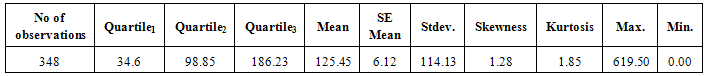
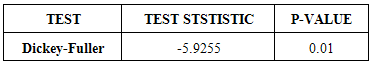
In this work the Ikeja monthly rainfall data from January, 1980 to December, 2012 was sourced from the central bank of Nigeria (CBN) official website [9] and we have extensively used R [10] to perform the analysis.In Fig.1 the Time series plot shows substantial periodicity (seasonality) and no trend while the Kernel density plot, box plot and the QQ-plot shows that the rainfall data is not normally distributed but positively skewed and heavy tailed as supported by the estimated skewness and kurtosis parameters in Table 1. To investigate the stationarity of the data we embark on a statistically significant test based on the Augmented Dickey-Fuller test [11] at 5% level of significance with hypothesis: H0: the time series data is unit root non stationary and H1: the time series data is stationary.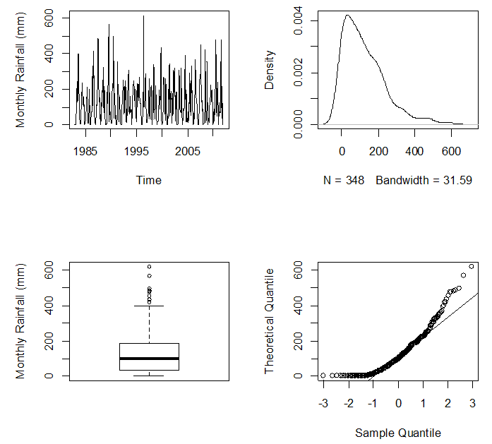 | Figure 1. Time series plot of Ikeja monthly rainfall (Top left panel), Kernel density plot of Ikeja monthly rainfall (Top right panel), Box plot of Ikeja rainfall (Bottom left panel) and QQ-plot of Ikeja monthly rainfal (Bottom right panel). Source of data: http//www.cbn.gov.ng |
Table 1. Descriptive statistics
 |
| |
|
Table 2. The Augmented Dickey-Fuller test
 |
| |
|
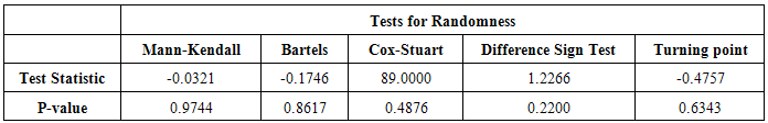
Decision: Small p-value less than 0.05 is in favour of the alternative hypothesis. Thus we reject the null hypothesis at 5% level of significance and conclude that the time series is stationary. The periodicity observed in the data has the consequence of violating the assumption of iid and thus could be remedied by subjecting the data to a seasonal differencing 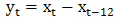 and the plot of the seasonally differenced data is shown in Fig.2.Also, various non parametric tests for randomness such as the Mann-Kendall rank test [12] and [13], Bartels rank test [14], Cox-Stuart test [15], Difference sign test [16], and Turning point test [16] were performed at 5% level of significance in R (using the package randtests) with the following hypothesis: H0: the data is random and H1: the data is non random. The results obtained are presented in Table 3.
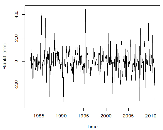 | Figure 2. Time series plot of the Ikeja seasonally differenced rainfall data. Source of data: http//www.cbn.gov.ng |
Table 3. Tests for Randomness
 |
| |
|
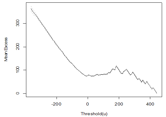 | Figure 3. Mean residual life plot |
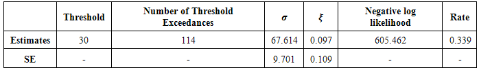
Decision: Since all the p-values are greater than 0.05 in favour of the null hypothesis we therefore retain the null hypothesis at 5% level of significance and conclude that the data is random hence, independent and identically distributed. To fit the Generalized Pareto distribution to the threshold excesses of the seasonally differenced rainfall series we first make a subjective choice of an appropriate threshold value from the mean residual life plot. The threshold value is chosen from where the mean residual life plot seems linear in the threshold  as shown in Fig. 3.Choosing a threshold of 30 from Fig. 3 we fit the generalized Pareto distribution to the exceedances (observations above the threshold) in R (using the package ismev) and the results are presented in Table 4.From the information provided in Table 4 it could be seen that a threshold of 30 provides 114 (exceedances) out of the 336 observations and the probability of exceeding the threshold is 0.339 and the positive value of the shape parameter
  implies a heavy tailed distribution for the exceedances while its large standard error of 0.109 (greater than the estimated parameter of 0.097) implies not significantly different from zero (0) at 5% level of significance. The diagnostic plots of the fitted model are shown in Fig. 4.From the diagnostic plots in Fig. 4 we could access the adequacy and validity of the fitted generalized Pareto distribution. Both the probability plot and the quantile plot depict a reasonable extreme value fit because, the probability plot is linear and the quantile plot is almost linear. The return level plot shows a slight convexity and the extreme values in the return level plot are within the 95% confidence bands and the density plot adequately fit the upper right tail of the distribution so the diagnostic plots do not raise any alarm on the adequacy and validity of the generalized Pareto fitting.
 Table 4. Parameter estimates of the fitted GP distribution
 |
| |
|
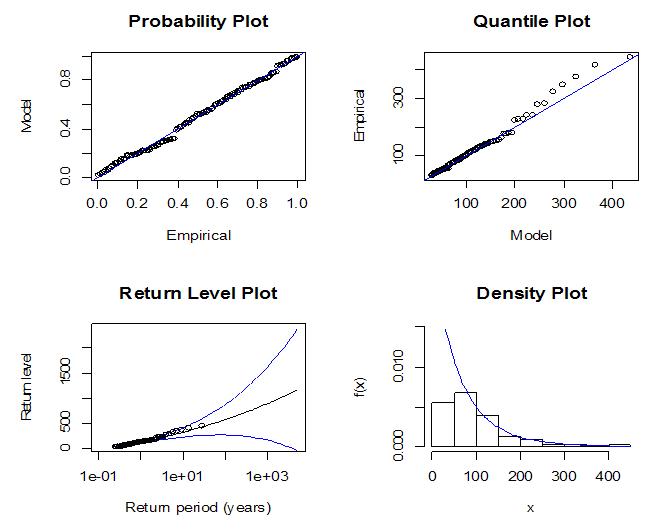 | Figure 4. Diagnostic plots of the fitted generalized Pareto (GP) distribution, threshold=30 |
4. Conclusions
The highest rainfall ever recorded in Ikeja since January, 1980 to December, 2012 is 691.50mm with an average rainfall of 125.45mm. The rainfall data shows substantial seasonality from the time series plot. A gross departure from normality was observed from the density, quantile and box plots. Also, the large positive values of the skewness (1.28) and kurtosis (1.85) parameters does not suggest otherwise. The generalized Pareto (GP) distribution was adequately fitted to the threshold excesses of the seasonally differenced rainfall data. The shape parameter  was found not significantly different from zero and the diagnostic plots lend full support on the adequacy and validity of the fitted GP model. The results obtained could serve as a guide to stakeholders in weather and climatic management.
Note
1. Threshold is a value that is used to determine a set of extreme values that follows a GPD. Threshold choice could be made by considering the plot of the threshold  against the mean excesses over the threshold given by
  which is a linear function of
  . However, the plot has the locus of points
  where
where  is the
  observations that exceeds
  and the plot is known as the mean residual life plot, [8].
References
| [1] | Efobi Kinsley and Anierobi Christopher Impact of flooding on Riverine Communities: The Experience of the Omabala and other Areas in Anambara State, Nigeria: Journal of Economic and Sustainable Development. - 2013. - 18 : Vol. 4. |
| [2] | Odunga S., Oyebande L. and Omojola A. S. Social-Economic Indicators and Public Perception on Urban Flooding in Lagos, Nigeria: Nigerian Association of Hydrological Sciences. - 2012. |
| [3] | Andrew Sibley Analysis of extreme rainfall and flooding in Cumbria 18-20 November 2009: Royal meteorological society. - 2010. - 11 : Vol. 65. - ISBN 9780954948016. |
| [4] | Fisher R. A. and Tippett L. H. C. Limiting forms of the frequency distribution of the largest or smallest member of a sample: Proceedings of the Cambridge Phylosophical Society. - 1928. - Vol. 24. - pp. 180-290. |
| [5] | Gnedenko B. Sur la distribution limite du terme maximum d'une serie aleatoire: Annals of Mathematics. - 1943. - Vol. 44. - pp. 423-453. |
| [6] | de Haan L. On Regular Variation and Its Application to the Weak Convergence of Sample Extremes Mathematical Centre Tract. - Amsterdam : Mathematisch Centrum, 1970. - Vol. 32. |
| [7] | Weissman I. Estimation of parameters and large quantiles based on the k largest observations: Journal of the American Statistical Association. - 1978. - Vol. 73. - pp. 812-815. |
| [8] | Coles Stuart An Introduction to Statistical Modelling of Extreme Values - London : Springer: Springer Series in Statistics, 2001. - p. 54. - ISBN 1-85233-459-2. |
| [9] | http//www.cbn.gov.ng |
| [10] | R Development Core Team R: A language and environment for statistical computing // R Foundation for Statistical Computing. - Vienna, Austria : [s.n.], 2014. - 3-900051-07-0. |
| [11] | Dickey D.A. and Fuller W.A. Distribution of the estimators for autoregressive time series with a unit root: Journal of the American Statistical Association , 1979. - Vol. 74. - pp. 427–431. |
| [12] | Mann H.B. Nonparametric test against trend: Econometrica. - 1945. - Vol. 13. - pp. 245-259. |
| [13] | Kendall M. Rank correlation methods: Oxford University Press, 1990. - 5th edition. |
| [14] | Bartels R. The Rank Version of von Neumann's Ratio Test for Randomness: Journal of the American Statistical Association. - 1982. - Vol. 77(377). - pp. 40-46. |
| [15] | Cox D. R. and Stuart A. Some quick sign test for trend in location and dispersion: Biometrika. - 1955. - Vol. 42. - pp. 80-95. |
| [16] | Mateus A. and Caeiro F. Comparing several tests of randomness based on the difference of observations. In T. Simos, G. Psihoyios and Ch. Tsitouras (eds.) : AIP Conf. Proc. 1558. - 2013. - pp. 809-812. |
 Abstract
 Reference
 Full-Text PDF
 Full-text HTML