Fernando Pongoh1, I Made Sumertajaya2, Muhammad Nur Aidi2
1Graduate student of Statistics Department, Bogor Agricultural University, Bogor, Indonesia
2Lecturer of Statistics Department, Bogor Agricultural University, Bogor, Indonesia
Correspondence to: Fernando Pongoh, Graduate student of Statistics Department, Bogor Agricultural University, Bogor, Indonesia.
| Email: |  |
Copyright © 2015 Scientific & Academic Publishing. All Rights Reserved.
Abstract
Poverty is a fundamental problem that existed and still occurs in Indonesia. This analysis was conducted to describe the factors that influence the welfare low status in sub-districts of North Sulawesi Province. Global regression has obtained influence variables to poverty status are woman leader in household (X1), Child not in formal education (X2), physical defect (X3), chronic desease victim (X5), self-owned house (X6), household using electricity (X8) and household using its own toilet (X10). Geographical weighted regression analysis (GWR) is a locally model, in order to estimates of parameters at each location. The result of GWR has different parameter estimation at each the location. Mix Geographical weighted regression model (MGWR) has combined local and global parameters. As well as the GWR, MGWR model results has give different parameter estimation at each location. GWR Model is the best model to explain the influence of the low welfare status in sub-districts of North Sulawesi Province which has the smallest value of MSE and AIC and the largest of R2 between Global Regression and MGWR.
Keywords:
Global Regression, Geographical Weighted Regression (GWR), Mix Geographical Weigthed Regression (MGWR)
Cite this paper: Fernando Pongoh, I Made Sumertajaya, Muhammad Nur Aidi, Geographichal Weighted Regression and Mix Geographichal Weighted Regression, International Journal of Statistics and Applications, Vol. 5 No. 1, 2015, pp. 1-4. doi: 10.5923/j.statistics.20150501.01.
1. Introduction
Poverty is a fundamental problem that existed and still occurs in Indonesian. The Economic crisis in 1998 gave a big problem to the national enonomy – increasing the number of the poors from 34.01 million (1996) to 49.50 million (1998) [1].Geographical weighted regression model with the function of normal kernel was the best model in explaining the average expenditure per capita per month in Jember sub-district [2]. Geographical weighted regression (GWR) was something that brought the framework of simple regression model to become weighted regression model [3]. The approach used was point approach in which every parameter value was measured in every geography location, therefore, every geography location spot had different regression coefficient value. In fact, in every situation not all regression coefficients from GWR model varied spaciously. The level of spatial diversity in some coefficients could not be significant, or it could be ignored. Consequently, GWR model was developed to the mix geographycal weighted regression (MGWR) in which it was the combination of linear regression model and GWR model, therefore, MGWR model could produce parameter estimation that had global parameter estimation, and other parameter that had local in accordance with its observation location. MGWR was better used to analyze the percentage of poor household in Mojokerto sub-district in 2008 [4].Tim nasional percepatan penanggulangan kemiskinan (TNP2K) is an institution established as the coordination organization of cross sector and cross functionary in central level to accelerate poverty tackling that has published welfare indicators in Indonesia provinces and integrated basic data in every sub-district, city or province. Based on the data basis, the analysis of the low welfare status in sub-districts of North Sulawesi Province would be performed by using GWR and MGWR analysis.
2. Research Method
The data used in this research were from integrated data basis to Social Protection Program July 2012 in 159 sub-districts of North Sulawesi Province. Moreover, latitude and longitude data were also used in every sub-district.Response variable (Y) is a low welfare status (%), while the predict variables were:X1: Woman leader in household (%)X2: Child not in formal education (soul)X3: Physical defect (%)X4: Patients with chronic diseases (%)X5: Chronic desease victim (soul)X6: self-owned house (%)X7: Households using protected water as water sources of drinking (%)X8: Household using electricity (%)X9: Households using gas cooking fuel/LPG/electricity (%)X10: Household using its own toilet (%)X11: Households using the final disposal of feces tank / SPAL (%)
3. Results
3.1. Global Regression
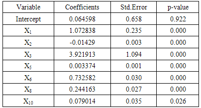
Global regression analysis obtained the influence variable of 5% level significant, i.e., woman leader in household (X1), Child not in formal education (X2), physical defect (X3), chronic desease victim (X5), self-owned house (X6), household using electricity (X8) and household using its own toilet (X10), shown in Tab1e 1. The variable Patients with chronic diseases (X4), households using protected water as water sources of drinking (X7), households using gas cooking fuel/LPG/electricity (X9) and households using the final disposal of feces tank / SPAL (X11) are not significant in that level. The value of R2 and adjusted-R2 are 0.969 and 0.967. In anova examination, it was obtained F value of 668.182 and F Table in the real level of 5% - the value of 2.05. This showed that regression model established gave significant influence towards the status data of low welfare in sub-districts of North Sulawesi Province.Table 1. Parameter Estimation of Global Regression
 |
| |
|
The examination of the assumption of the remaining normality that used kolmogorov smirnov test in the variable of low welfare status (Y) produced KS value of 0.49 with the value of p 0.97 at the real level of 5%. It showed that the spread of the remaining data was normal. The examination of multicolinierity was perfomed by considering the value of Variance Inflation Factor (VIF). The result of VIF showed that the variables had no strong correlation. It indicated that the VIF value in every variable was under 10. The examination of the homogeneity of variation was done exploratively, i.e. by considering the plot between y-assumption and the rest. The plot showed that the data formed the funnel-like pattern that indicated the variation homogeneity violation.The test of spatial variation that used Breusch-Pagan (BP) test yielded the BP value of 24.843 with the value-p of 0.000809 at the real level of 5%. This showed that there was spatial variation at the status data of low welfare in sub-district of North Sulawesi Province. The variation of spatial indicated that every sub-district in North Sulawesi Province had its own characteristics, therefore, the local approach was needed to modelize and overcome the variation that happened in low welfare status.
3.2. Geographically Weighted Regression (GWR)
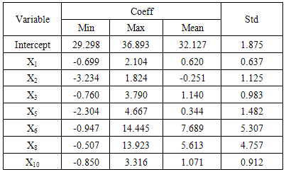
At the analysis of the first step of GWR which was performed determined the value of optimum bandwith with iteration to get minimum cross-validation. The result of iteration yielded minimum cross-validation of 5.119 with bandwith value of 42.855. This bandwith value described that the distance limit in an area where the distance was under 42.855 km gave more influence compared to that of above 42.855 km. The weighted matrix was formed by using the function of adaptive bisquare: Wij = (1 – dij2/42.855)2. Table 2. Summary Estimation Parameter of GWR Model
 |
| |
|
The coefficients parameter of variable X1, X2, X3, X5, X6, X8 and X10 was shown in Table 2. Model of GWR got the value of R2 0.994 and adjusted-R2 0.989. The examination of GWR anova resulted in the value of F-calculation of 6.086, meanwhile the value of table F that was in the real level of 5% was 1.48. This indicated that there was a significant difference between global regression model and GWR model. GWR model give different estimation parameter in every sub-district, Table 3 shown estimation parameter at Posigadan sub-district and Maesa sub-district.The significant variable (α = 5%) at Posigadan sub-district are physical defect (X3), self-owned house (X6), household using electricity (X8) and household using its own toilet (X10). GWR model Y= 34.977 + 2.219X3 + 12.345X6 + 1.711X10 and R2 0.986.The other, Maesa sub-district significant variable (α = 5%) are woman leader in household (X1), self-owned house (X6), household using electricity (X8) and household using its own toilet (X10). GWR model Y = 35.208 + 1.678X1 + 8.468X6 + 2.597 X8 + 2.988 X10 and R2 0.983.Table 3. Estimation Parameter of GWR Model at Posigadan and Maesa
 |
| |
|
3.3. Mix Geographically Weighted Regression (MGWR)
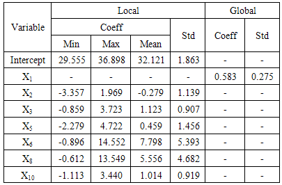
The initial step in MGWR that determined the local and global variables yielded the variables of Child not in formal education (X2), physical defect (X3), chronic desease victim (X5), self-owned house (X6), household using electricity (X8) and household using its own toilet (X10) as the local variable; and woman leader in household (X1) variable as the global variable. The value of Bandwith obtained the value of 42.855 with the cross-validation of 4.956. The value of bandwith described that the distance limit in an area in which the distance was under 42.855 km gave more influence compared to that of above 42.855 km. The weighted matrix was formed by using the function of adaptive bisquare: Wij = (1 – dij2/42.855)2.The local parameter and global parameter estimation was shown in Table 4. MGWR model obtained the value of R2 0.993 and adjusted-R2 0.989. The examination of anova indicated the value of F-calculation of 6.546, meanwhile the value of table F in the real level of 5% was 1.50. This showed that there was significant difference between the global regression model and MGWR model. MGWR model give different estimation parameter in every sub-district, Table 5 shown estimation parameter at Posigadan sub-district and Maesa sub-district.Table 4. Summary Estimation Parameter of MGWR Model
 |
| |
|
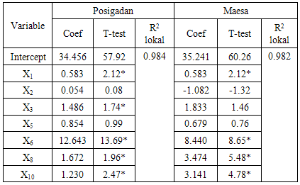
The significant variable (α = 5%) at Posigadan sub-district are woman leader in household (X1), physical defect (X3), self-owned house (X6), household using electricity (X8) and household using its own toilet (X10). MGWR model Y= 34.456 + 0.583X1 + 1.486X3 + 12.643X6 + 1.230X10 and R2 0.986.The other, Maesa sub-district significant variable (α = 5%) are woman leader in household (X1), self-owned house (X6), household using electricity (X8) and household using its own toilet (X10). MGWR model Y = 35.241 + 0.583X1 + 8.440X6 + 3.474 X8 + 3.141 X10 and R2 0.982.Table 5. Summary Estimation Parameter of MGWR Model
 |
| |
|
3.4. Compare of Regression Global, GWR and MGWR
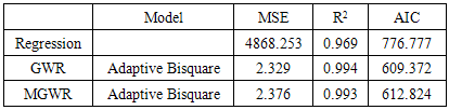
The global regression model, GWR model and MGWR model were compared with the value of MSE, AIC and R2 from every model. The model with the smallest MSE and AIC values and the biggest value of R2 was the best model. Table 6 showed that the smallest MSE and AIC values were 2.329 and 609.372 at GWR model. The biggest value of R2 was also owned by GWR model of 0.984. Therefore, it could be concluded that GWR model was the best model in explaining the influence towards the low welfare status in sub-district of North Sulawesi Province.Table 6. Compare of Regression, GWR and MGWR
 |
| |
|
4. Conclusions
The influencing factors of low welfare status in sub-districts of North Sulawesi Province using global regression analysis are woman leader in household (X1), the number of Child not in formal education (X2), physical defect (X3), chronic desease victim (X5), self-owned house (X6), household using electricity (X8) and household using its own toilet (X10).In each sub-district could be obtained the different influencing factors of low welfare using GWR analysis. In the case, influence factors at posigadan sub-district is not equal with influence factors at Maesa sub-districs. The influence factors at Posigadan sub-district are physical defect (X3), self-owned house (X6), household using electricity (X8) and household using its own toilet (X10). At Maesa sub-district, the influence factors are woman leader in household (X1), self-owned house (X6), household using electricity (X8) and household using its own toilet (X10).
References
| [1] | BPS, Statistik Indonesia: Statistical Year Book of Indonesia, 2014. |
| [2] | Rahmawati R, “Model Regresi Terboboti Geografis dengan Pembobot Kernel Normal dan Kernel Kuadrat Ganda untuk Data Kemiskinan: kasus 35 desa atau kelurahan di kabupaten jember,” thesis. Institut Pertanian Bogor, Bogor, Indonesia. 2010. |
| [3] | Fotheringham AS, Brunsdon C, Chartlon M, Geographically Weighted Regression, the Analysis of Spatially Varying Relationships, John Wiley and Sons, LTD. 2002. |
| [4] | Purhadi dan Yasin H, 2012, Mixed Geographically Weighted Regression Model, Case Study: the Precentage of Poor Households in Mojokerto 2008, European Journal of Scientific Research, 69(2), 188-196. |
 Abstract
 Reference
 Full-Text PDF
 Full-text HTML