Michael Asamoah-Boaheng
School of Graduate Studies Research and Innovation, Kumasi Polytechnic, Kumasi, Ghana
Correspondence to: Michael Asamoah-Boaheng, School of Graduate Studies Research and Innovation, Kumasi Polytechnic, Kumasi, Ghana.
| Email: |  |
Copyright © 2014 Scientific & Academic Publishing. All Rights Reserved.
Abstract
Meteorologists actually use a combination of several different mathematical methods to come up with their periodical weather forecasts for phenomena such as average temperature, rainfall, humidity and other atmospheric conditions. Using Seasonal Autoregressive Integrated Moving Average (SARIMA) model, the study determined an adequate forecasting model for the mean temperature of Ashanti Region with data from the Department of Meteorology and Climatology from the period of 1980 to 2013. The following SARIMA: SARIMA(2,0,2)(2,1,1)(12), SARIMA(2,1,1)(1,1,2)(12) and SARIMA(1,1,1) (1,1,1)(12) with BIC of 502.36, 522.44, 492.73 and 495.92 respectively were obtained and compared. SARIMA (2,1,1)(1,1,2)(12) had the least BIC and was considered the adequate model for prediction. They however recorded a ME, RMSE, MAE, MPE, MAPE, MASE of 0.012, 0.516, 0.382, 0.006, 1.408 and 0.419 respectively. The residuals of the model were white noise of passing Ljung-Box at 5 percent with p-values (0.7809).
Keywords:
Meteorologists, Average temperature, Box Jenkins, Seasonal components
Cite this paper: Michael Asamoah-Boaheng, Using SARIMA to Forecast Monthly Mean Surface Air Temperature in the Ashanti Region of Ghana, International Journal of Statistics and Applications, Vol. 4 No. 6, 2014, pp. 292-298. doi: 10.5923/j.statistics.20140406.06.
1. Introduction
This study investigated the general pattern of mean temperatures recorded in Ashanti Region from 1980 to 2013 and developed Seasonal Autoregressive Integrated Moving Average (SARIMA) forecast model for predicting 2014 mean monthly temperature. Temperature is a physical quantity that is a measure of hotness and coldness on a numerical scale. It is a measure of the thermal energy per particle of matter or radiation and it is measured by a thermometer, which may be calibrated in any of various temperature scales [6]. Temperature is an intensive property, which is independent of the amount of material present and in contrast to energy, an extensive property, which is proportional to the amount of material in the system. Time series analysis of mean temperature based on air temperature data obtained from State Meteorological Service in Turkey between 1950-1994 was investigated by [2]. Regional changes were observed in the mean temperatures in Turkey from 1950-1994. Also the study observed a statistically significant cooling trend in 21 stations as well as warming trend in one station and no trend in 36 stations.[4] applied SARIMA on hourly bicycle count and temperature data and modeled Vancouver Bicycle Traffic using weather variables. Complex serial correlation patterns in the error terms and model tests against actual bicycle traffic counts were accounted by the ARIMA model. [5] investigated into weather variability and the incidence of cryptosporidiosis; comparison of time series poisson regression and SARIMA models. They performed time series Poisson regression and (SARIMA) models in examining the potential impact of weather variability on the transmission of cryptosporidiosis. Model assessment showed SARIMA model having better predictive ability than the Poisson regression model (SARIMA: root mean square error (RMSE): 0.40, Akaike information criterion (AIC): -12.53; Poisson regression: RMSE: 0.54, AIC: -2.84).[7] researched into the relationship between Weather Temperature and Mortality; A Time Series Analysis Approach in Barcelona. They estimated several transfer function (ARIMA) models for the entire period and for both winters and summers separately. At least three consecutive days of increased weather temperature resulted in an increase in mortality and the discovery of an independently V-shaped relationship. [8] conducted a comparative study of statistical and neuro-fuzzy network models for forecasting the weather of Goztepe, Istanbul, Turkey using ANFIS and Autoregressive Integrated Moving Average (ARIMA) models. A nine year data (2000-2008) was used comprising daily average temperature, air pollution and wind speed. The performance of ANFIS and ARIMA after comparison was evaluated due to MAE, RMSE, R2 criteria with ANFIS giving better results.
2. Materials and Methods
Time series is a time dependent sequence Yt, where t belongs to the set of integers and denotes the time steps. If a time series can be expressed as a known function, Yt= f (t), then it is said to be a deterministic time series. If it is however expressed as Yt= X (t), where X is a random variable then {Yt} is a stochastic time series.
2.1. Data Used
Secondary data from the Department of Meteorology and Climatology in the Ashanti Region from the period of 1985 to 2013 was used to develop a forecast model (SARIMA) in predicting future mean temperature values in Ashanti Region of Ghana. The data was used since it is a time series data and the observations were collected sequentially in time (monthly). Data was analysed with R-Console V. 2.15.1.
2.2. Stationary and Non Stationary Series
A time series is said to be strictly stationary if the joint distribution of Xt1, Xt2,… Xtn is the same as the joint distribution of Xt1+T, Xt2+T,…Xtn+T for all X1+T…Xn+T. Thus, shifting the time position by T periods has no effects on the joint distributions, which therefore depends on the interval between t1… tn. If a time series is not stationary then it is said to be non-stationary. A simple non-stationary time series model is given by  | (1) |
Where the mean  is a function of time and
  is a weakly stationary series.
2.2.1. Unit Root Test
Unit Root Test was derived in 1979 by Dickey and Fuller to test the presence of a unit root vs. a stationary process. The unit root process and a stationary process are given by equations 3.1 and 3.2 below; | (2) |
 | (3) |
If =1 then the series is said to have unit root and is not stationary. The Unit Root Test as proposed by Kwiatkowski-Phillips-Schmidt-Shin (KPSS), test the hypothesis below: H0: Φ1=series is level or trend stationaryHA: Φ1=series is level or trend non-stationaryIf test statistic value of the KPSS test is less than critical value, we accept the null hypothesis that the data is level or trend stationary. Similarly, the Unit Root Test as proposed by Dickey and Fuller (ADF), test the hypothesis below:H0: Φ1=series has unit rootHA: Φ1=series has no unit rootIf test statistic of the ADF test is less than critical value we reject the null hypothesis that the data has a unit root.
2.3. ARIMA Models
The acronym ARIMA stands for "Auto-Regressive Integrated Moving Average." Lags of the differenced series appearing in the forecasting equation are called "auto-regressive" terms, lags of the forecast errors are called "moving average" terms, and a time series which needs to be differenced to be made stationary is said to be an "integrated" version of a stationary series. A non-seasonal ARIMA model is classified as an "ARIMA (p, d, q)" model, where p is the number of autoregressive terms, d is the number of non-seasonal differences, and q is the number of lagged forecast errors (moving average) in the prediction equation. A process,  is said to be ARIMA (p, d, q) if
 | (4) |
is ARMA (p, q). In other words the process should be stationary after differencing a non-seasonal process d times. In general, we will write the model as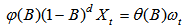 | (5) |
If we let  We write the model as
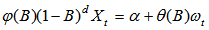 | (6) |
Where 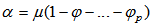
2.4. The Box-Jenkins ARIMA Model
The Box-Jenkins methodology refers to the set of procedures for identifying, fitting, and checking ARIMA models with time series data. Forecasts follow directly from the form of the fitted model. By Box-Jenkins, a pth order autoregressive model: AR (p), has the general form | (7) |
Where Xt = Response (dependent) variable at time t, Xt-1 , Xt-2,… Xt-p = Response variable at time lags t−1, t−2,. . . t−p, respectively. 1, 1,…, p = Coefficients to be estimated, and  term at time t. Also, a qth- order moving average model: MA (q), has the general form
 | (8) |
Where Xt= Response (dependent) variable at time t, µ= Constant mean of the process, 1, 1,…, p=Coefficients to be estimated,  term at time t, and ωt-1, ωt-2, ωt-p=Errors in previous time periods that are incorporated in the response Xt.Autoregressive Moving Average Model: ARMA (p, q), which has the general form
 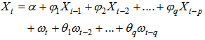 | (9) |
(We can use the graph of the sample autocorrelation function (ACF) and the sample partial autocorrelation function (PACF) to determine the model which processes are summarized as follows:| Table 1. How to determine the model by using ACF and PACF patterns |
| | MODEL | ACF | PACF | | AR (p) | Dies down | Cut off after lag q | | MA (q) | Cut off after lag p | Dies down | | ARMA (p, q) | Dies down | Dies down |
|
|
Box-Jenkins forecasting models consist of a four-step iterative procedure as follows; Model Identification, Model Estimation, Model Checking (Goodness of fit) and Model Forecasting.
2.5. The Box Jenkins Seasonal (SARIMA) Model
[1] have generalized the ARIMA model to deal with seasonality and define a general multiplicative seasonal ARIMA model (abbreviated SARIMA model) as 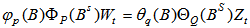 | (10) |
Where B denotes the backward shift operator,  are polynomials of p,P,q,Q respectively, Zt denotes a purely random process, and
  | (11) |
This model looks rather complicated at first sight, however if P=1, then the term  will be (1-constant x Bs), which simply means Wt will depend on Wt-s, since Bs Wt = Wt-s. The variable {Wt} are formed from the original series {Xt} not only by simple differencing but also by seasonal differencing,
  to remove seasonality. For example if d=D=1 and s=12, then
 The model in equations 10 and 11 is said to be a SARIMA model of order (p,d,q) X (P,D,Q). The model values of d and D do not usually need to exceed one. [3]. For instance, considering a SARIMA model of order (1,0,0) x (0,1,1)12 then equations 10 and 11 can be rewritten as
 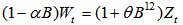 Where
Where  then we find
3. Results and Discussion
3.1. Pattern of the Mean Temperature Recorded from January 1980 to December 2013
This section discusses the analyses of the results following the Box-Jenkins Approach in model building. Figure 1 below shows the mean temperatures recorded over the years from January 1980 to December 2013.The series shows no particular trend, hence appears stationary since the series is constant in size over time. The series shows generally the rise and fall of mean temperatures over the years. But by critical observations year by year, it is clear that, there existed a sharp rise and fall in the mean temperatures recorded. However the highest mean temperature was recorded in the year 1984 (i.e. above 300C) and the least recorded around 1983.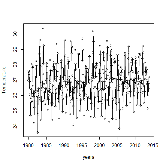 | Figure 1. Time series Plot of Mean temperature recorded from Jan. 1980-Dec. 2014 |
Figure 1 above was further decomposed to observe the various components in the series. Figure 2 below shows the decomposed mean temperature with respect to the various years recorded.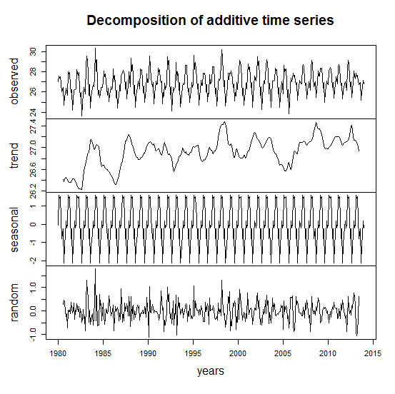 | Figure 2. Decomposed time series plot of mean temperatures |
From Figure 2 we observed existence of seasonal variation in the series which is constant over time, the random effect also constant over time and the pattern (trend) of the series which seems stationary and also constant over time. Also from observation, seasonal effect/variation occurred every year or every twelve month period from 1980 through to 2013. In other words, regular mean temperatures are recorded each year due to the rise and fall of mean temperatures in each year at regular times.
3.2. Fitting an ARIMA Model of the Series Using the Box-Jenkins Approach
Box-Jenkins forecasting models consist of a four-step iterative procedure as follows; Model Identification, Model Estimation, Model Checking (Goodness of fit) and Model Forecasting.
3.2.1. Model Identification
The model development process begins by studying the original plot, ACF, PACF and objective test of the raw data to be sure that it is stationary. To ensure that the series plotted in Figure 1 was stationary, ACF and PACF were plotted after observing a constant variance in the mean temperature. Figure 3 shows the sample ACF and PACF of the mean temperature series with 95% confidence limits. From the correlogram, most of the spikes in both the ACF and the PACF were observed to be outside the confidence limits. Also the ACF shows a cyclic or seasonal movement/variation of the correlations, hence shows sinusoidal waves and oscillation movements. Also both the ACF and the PACF shows slow decay of the spikes indicating that the series has no trend and hence stationary.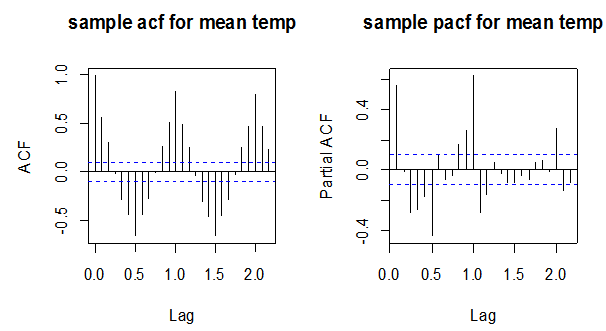 | Figure 3. Figure: 1.3: Sample ACF and PACF of the series (mean temperatures) |
Also, Kwiatkowski-Phillips-Schmidt-Shin (KPSS) and Augmented Dickey- Fuller (ADF) test from Table 2 were performed. From Table 2, the KPSS test with p-value of 0.1 and ADF test with p-value of 0.01 proved the stationarity of the temperature series in Figure 1.| Table 2. Objective test (unit root test) for drift and trend stationarity of mean temperature |
| | TEST TYPE | Test statistic | P-value | | ADF | -11.3867 | 0.01 | | KPSS | 0.2038 | 0.1 |
|
|
KPSS Test for Level StationarityHo: There is level Stationarity H1: There is no level StationarityADF test Ho: There is no Stationarity H1: The series is stationary. Next is to difference the series to remove the seasonal components in the series in order to determine the orders/values of the non-seasonal and the seasonal AR and MA parts. Figure 4 gives the ACF and the PACF of the one regular differenced seasonal series.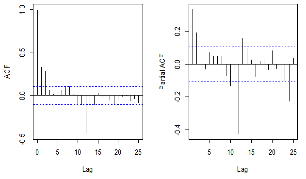 | Figure 4. ACF and PACF of one seasonal differencing |
From Figure 4 above, the ACF (at low lags) i.e. at lags 1 and 2 are significantly different from zero since the spikes passes out of the confidence limits. Hence the order of the non-seasonal MA term is 2 and that of the seasonal MA terms occurs at lags which are multiples of 12. Only one spike is significant at lag 12. Hence the order of seasonal MA term is 1. Similarly, significant spikes in the PACF (at low lags) indicated possible non-seasonal AR terms. The order of the non-seasonal AR part is 2 and that of the seasonal AR is 2.This therefore suggests an arima model in the form SARIMA (2, 0, 2) (2, 1, 1) (12).
3.2.2. Model Estimation and Evaluation
The procedure for choosing these models relies on choosing the model with the minimum AIC, AICc and BIC. The models are presented in Table 3 below with their corresponding values of AIC, AICc and BIC. | Table 3. AIC, AICc and BIC for the Suggested ARIMA Models |
| | MODEL | AIC | AICc | BIC | | SARIMA (2,0,2)(2,1,1)(12) | 471.54 | 471.97 | 502.36 | | SARIMA (1,1,2)(1,0,1)(12) | 499.14 | 499.37 | 522.44 | | SARIMA (2,1,1)(1,1,2)(12) | 465.78 | 466.11 | 492.73 | | SARIMA (2,0,1)(2,0,0)(12) | 576.07 | 576.39 | 603.27 | | SARIMA (1,1,1)(1,1,1)(12) | 476.67 | 476.85 | 495.92 | | SARIMA (2,0,0)(2,0,0)(12) | 575.13 | 575.37 | 598.45 |
|
|
From Table 3, the model with the least AIC, AICc and BIC is SARIMA (2,1,1)(1,1,2)(12) indicating that SARIMA (2,1,1)(1,1,2)(12) is the best model for predicting the mean temperature of Ashanti Region.
3.2.3. Goodness of fit/Model Verification/Model Diagnostics
In time series modeling, the selection of a best model fit to the data is directly related to whether residual analysis is performed well. One of the assumptions of SARIMA model is that, for a good model, the residuals must follow a white noise process. That is, the residuals have zero mean, constant variance and also uncorrelated.| Table 4. Parameter estimation of the appropriate model (SARIMA (2, 1, 1) (1,1,2)(12)) |
| | | ar1 | ar2 | ma1 | sar1 | sma1 | sma2 | | Coefficients | 0.3033 | 0.1726 | -0.9904 | -0.586 | -0.344 | -0.551 | | SE | 0.0508 | 0.0507 | 0.0168 | | | | | | | ME | RMSE | MAE | MPE | MAPE | MASE | | | 0.0119 | 0.5157 | 0.3818 | 0.0060 | 1.4076 | 0.4189 | |
|
|
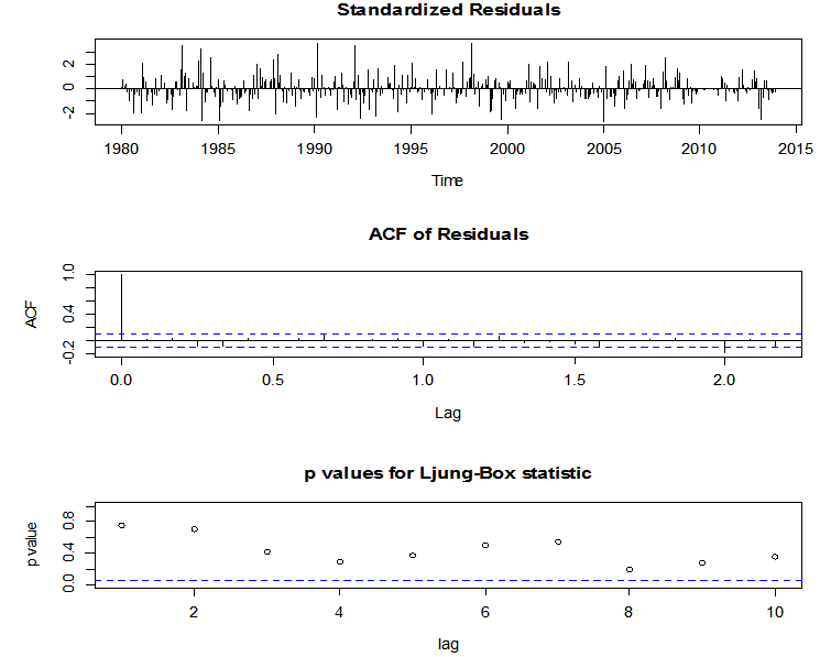 | Figure 5. Plots of model residuals of mean temperatures recorded from 1980 to 2013 |
From Figure 5 above, the standardized residual shows that the residuals of the model have zero mean and constant variance since the residuals are concentrated around -2 to 2. Also the ACF of the residuals of the model shows that the autocorrelation of the residuals are all zero, that is to say they are uncorrelated, hence the residuals assume mean of zero and constant variance, hence they are uncorrelated. Finally, the p-value (0.7809) for the Ljung-Box statistic in the third panel in Figure 5 all clearly exceed 5% for all lag orders, indicating that there are no significant departure from white noise for the residuals. Thus, the selected model “SARIMA (2, 1, 1) (1, 1, 2) [12]” satisfies all the model assumptions.
3.2.4. Normality Test for Residuals
Figure 6 shows the normality test plots of the model residuals. From the Q-Q plot, it can be observed that, most of the points passes through the straight line with few of the points very closed to the straight line. This shows that the residuals in the model are normal. From the histogram plot of residuals on the left of Figure 6, the distribution of the residuals can be clearly seen as normal having a bell shape distribution. Therefore SARIMA (2,1,1)(1,1,2)(12) satisfies all the model assumptions indicating that the model is very good for forecasting.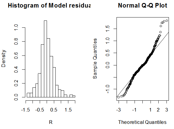 | Figure 6. Plots of normality test for model residuals |
3.2.5. Forecasting using SARIMA (2,1,1)(1,1,2) [12]
Using the derived model, the following forecast were made for the year 2014 as shown in Table 5 with lower and upper limit forecast.| Table 5. Forecasted values for 12 months mean temperatures for 2014 |
| | | | | Confidence Limits | | Year | Month | Forecast | lower | Upper | | 2014 | January | 27.02 | 26.16 | 27.87 | | | February | 28.56 | 27.66 | 29.46 | | | March | 28.56 | 27.63 | 29.49 | | | April | 28.60 | 27.66 | 28.54 | | | May | 27.45 | 26.51 | 28.39 | | | June | 26.43 | 25.48 | 27.37 | | | July | 26.94 | 26.01 | 27.89 | | | August | 25.07 | 24.12 | 26.02 | | | September | 26.01 | 25.07 | 26.96 | | | October | 26.64 | 25.69 | 27.59 | | | November | 27.42 | 26.47 | 28.36 | | | December | 27.03 | 26.08 | 27.98 |
|
|
4. Conclusions
The pattern of mean temperatures in Ashanti Region from 1980 to 2013 was observed to be stationary, hence does not follow any particular pattern (neither increasing nor decreasing). The stationarity of the mean temperature series was verified by the plot of the sample ACF and PACF’s as well as the use of KPSS and ADF tests. The highest mean temperature (i.e. above 30oC) was recorded in 1984. However regular mean temperature values were recorded every year, hence the presence of seasonal components were observed through the decomposition of the series.The seasonal component of the series was removed through one regular differencing. Following the procedures of the Box Jenkin’s SARIMA model building, several suggested models were developed. However based on the computed AIC, AICc, BIC values for each of the suggested models, the best model was derived as SARIMA (2,1,1)(1,1,2)(12). However, model diagnostics were performed through careful performance of the model residuals. The model residuals were found to be following a white noise process with a mean of zero and a constant variance, hence uncorrelated. Also the model residuals were found to be near normality through the plots of histograms and Q-Q plot. Based on the model diagnostics performed, the identified model was found to be very adequate and good for predicting future mean temperatures in Ashanti Region. The forecasted mean temperature values showed similar pattern of previous recordings.
References
| [1] | Box, G.E.P., and Jenkins, G.M., 1970, Time Series Analysis, forecasting and control, Englewood cliffs, NJ:Prentice Hall, 3rd ed. |
| [2] | Can, A., and Atimtay, A.T., 2002, Time series analysis of mean temperature data in turkey, Applied Time series, 4, 20-23. |
| [3] | Chatfield, C., 1995, The Analysis of Time Series: An introduction. Chapman and Hall, Washington D.C, New York. (5thed). |
| [4] | Gallop, C., Tseand, C., Zhao, J., 2012, A Seasonal Autoregressive Model of Vancouver Bicycle Traffic Using Weather Variables.TRB 2012 Annual Meeting. |
| [5] | Hu, W., Tong, S., Mengersen, K., and Connel, D., 2010, Weather Variability and the Incidence of Cryptosporidiosis: Comparison of Time Series Poisson Regression and SARIMA Models. 51(1). |
| [6] | Maxwell, J.C., 1871, Theory of Heat, Longmans, Green, and Co., London. p. 2. |
| [7] | Saez, M., Sunyer, J., Castellsague, J., Murillo, C., and Manto, J., 1994, Relationship between Weather Temperature and Mortality: A time series analysis approach in Barcelona. International Journal of Epidemiology, 24 (3), Pages 576-582. |
| [8] | Tektax, M., 2010, Weather Forecasting Using ANFIS and ARIMA Models: A Case Study for Istanbul. Environmental Research, Engineering and Management, 1(51), Pages 5-10. |
 Abstract
 Reference
 Full-Text PDF
 Full-text HTML