-
Paper Information
- Next Paper
- Previous Paper
- Paper Submission
-
Journal Information
- About This Journal
- Editorial Board
- Current Issue
- Archive
- Author Guidelines
- Contact Us
International Journal of Statistics and Applications
p-ISSN: 2168-5193 e-ISSN: 2168-5215
2014; 4(6): 249-268
doi:10.5923/j.statistics.20140406.02
Statistically Significant Relationships between Returns on FTSE 100, S&P 500 Market Indexes and Macroeconomic Variables with Emphasis on Unconventional Monetary Policy
 Abstract
 Reference
 Full-Text PDF
 Full-text HTML
Aweda Nurudeen Olawale1, Are Stephen Olusegun2, Akinsanya Taofik1
1Department of Statistics, Yaba College of Technology, Nigeria
2Department of Statistics, Federal Polytechnic, Ilaro, Nigeria
Correspondence to: Aweda Nurudeen Olawale, Department of Statistics, Yaba College of Technology, Nigeria.
| Email: |  |
Copyright © 2014 Scientific & Academic Publishing. All Rights Reserved.
Establishing the nature of relationships between macroeconomic variables and stock market returns are imperative to investors and understanding the stock market dynamics in any country. These relationships have been extensively studied in both emerging and the developed stock markets. By employing vector error correction and cointegration techniques, this current study established the statistically significant long-run and short-run causal relationships between macroeconomic variables and the stock market returns of FTSE100 and S&P500 stock market indexes in the United Kingdom and United States respectively. The macroeconomic variables employed include industrial production index, short-term interest rates, exchange rates, consumer price index and unemployment rates in addition to broad money supply M3 that was included as an exogenous variable. Also global financial crisis was introduced, as a dummy variable to capture structural breaks inherent in the data. Empirical results showed that significant long-run relationship existed between stock market returns and industrial production index, interest rates, and consumer price index in the United Kingdom while stock market returns in the United States was influenced by all variables except industrial production index. Furthermore, results indicated that it takes longer for stock market returns to adjust to its long-run equilibrium in the UK than in the US. In the short-run, industrial production index, short-term interest rates, and unemployment rates have no significant causal link with returns on FTSE100. Similarly, industrial production index and exchange rates have no significant short-run causality with returns on S&P500. Unconventional monetary policies (Quantitative Easing or Large-Scale Assets Purchases) adopted by Federal Reserve have positive impact on the S&P500 stock market returns.
Keywords: Vector Error Correction, Cointegration, FTSE100, S&P500, Long-run, Equilibrium, Quantitative Easing, Financial Crisis
Cite this paper: Aweda Nurudeen Olawale, Are Stephen Olusegun, Akinsanya Taofik, Statistically Significant Relationships between Returns on FTSE 100, S&P 500 Market Indexes and Macroeconomic Variables with Emphasis on Unconventional Monetary Policy, International Journal of Statistics and Applications, Vol. 4 No. 6, 2014, pp. 249-268. doi: 10.5923/j.statistics.20140406.02.
Article Outline
1. Introduction
- Financial market divided primarily into market for short-term funds (money market) and long-term financial assets (capital market) play an important role in the economy by linking individuals and firms, serving as a mechanism for mobilization and allocation of savings into investments. The capital market can be subdivided into primary market where new financial securities are issued and secondary market (otherwise referred to as stock market) for trading existing negotiable financial securities (stocks). Thus, the existence of a stock market makes trading of securities possible thereby making funds available for investment purposes in an economy. Macroeconomic variables such as money supply, interest rates (long-term and short-term), inflation rates, level of output (industrial production, employment level), exchange rates, alongside external forces, government structure and firms’ profitability through demand and supply determine the price at which stocks are bought or sold on the stock exchange. Consequently, establishing the nature of the relationship between macroeconomic variables and stock market returns is imperative to investors and understanding the stock market dynamics in any country. These relationships have been extensively studied in both emerging and the developed stock markets. Monetary policy interacts with the economy via transmission channel through the purchase and sale of bonds only. It can also influence the economy through the purchase of goods and services as well as financial assets such as treasury bills and common shares. Monetary policy is used by monetary authorities particularly the central banks to majorly achieve potential production through full employment, eliminate budget deficit (balance of payment deficit), realize economic growth and reduce the rate of inflation. According to the quantity theory of money, it is widely accepted that the money supply affects only the level of prices in an economy. However, its failure during the period of the great depression in the 1930s led to its abandonment. An alternative school of thought, Keynesian theory, proposed that the stock of money could be controlled by central banks such as the Bank of England and Federal Reserve. This theory also proposed that the demand for money is determined by gross national income and the rate of interest. And that the restoration of equilibrium between the demand for and supply of money is achieved through the financial assets markets. Contrary to quantity theory, Keynesian theory hypothesizes that change in the money supply cause changes in the rate of interest and not the inflation rate. Consequently, Milton Friedman in the 1950s introduced monetarism by modifying the quantity theory of money stating that economic systems have the inclination of moving towards full employment equilibrium. He claimed that in the long-run, the supply of money will have an effect on the inflation. Monetarism asserts that financial assets bear yield or return inform of interest payment (Hanson, 1983). This theory considers money as having a limited effect on demand for financial assets including bonds and stocks. According to Global Financial Stability Report (2012), “monetary policies play an important role in smoothing economic activity and influence the functioning of financial intermediation and financial structure”. Under normal situation, expansionary policy (contractionary policy) leads to increase (decrease) in production and inflation rates resulting in higher (lower) interest rates. Higher (lower) interest rates leads to reduction (increase) in current consumption and investment. However, nominal interest rate may get close to zero during period of recession which results in the transmission channel becoming inexistent and making production shock greater due to continuous attempts by the central banks to further bring down nominal interest rate (Auerbach, 2012). Therefore, excess liquidity as a consequence of unconventional monetary policy such as quantitative easing (QE)1 or Large-Scale Assets Purchase (LSAPs) by central banks result in increase in asset prices and lower interest rates which in turn lead to higher rate of return. LSAPs involve purchase of treasury and government sponsored enterprises (GSEs) to stimulate the economy through lower long-term interest rates. Bridges and Thomas (2012), iterated given the store of value function of money, the demand for broad money hinges on the nominal expenditure on goods and services, the value of asset transactions, value of overall asset portfolios and the relative rate of return on money. Stocks (financial asset) are good substitutes for money (for a great number of investors) especially when the rate of return is high. Theoretically, the marginal rate of substitution between money now and other forms of security (stocks inclusive) now equals the current price of the security (Hicks, 1968). With a close dependence of the demand for money upon the rate of interest rate, increased money supply may lead to higher inflation and thereby increased nominal interest rate. Higher interest rates lead to higher required rate of return and lower stock prices. Rapach (2002) argued that increase in inflation does not necessarily result in persistent depreciation of real value of stock in the industrialized countries. Many literatures criticise the claim that the existence of a negative relationship between inflation and stock returns is as a result of increase in rate of inflation which is accompanied by both lower expected earnings growth and higher required real return. According to Fama (1981), significant relationship exists between macroeconomic variables such as industrial production index, GNP, money supply, inflation, interest rates and stock prices. He found strong positive correlations between common stock returns and these macroeconomic variables. Subsequently, several empirical studies have explored this area to ascertain the fundamentals of these relations in one country or in a group of countries. For example Chen et al. (1986) studied how some macroeconomic variables explain the US stock market movement using the Arbitrage Pricing Theory. Other researchers such as Cheung and Ng (1998), Mukherzee and Naka (1998) employed cointegration analysis to examine the relationships between stock returns and macroeconomic variables in developed economies such as Australia, Japan, US and Germany. The industrial production index is used as a measure of real economic activity in a country. Theoretically, the industrial production increases during expansionary business cycle and decreases during a contraction. Therefore, a change in industrial production would indicate a change in economy. During economic growth, the productive capacity of firms to generate future cash flows is greatly influenced, hence a positive relationship between real economy and stock prices exist. Fama (1981) showed that the growth rate of industrial production have a strong long-run relation with stock returns. Forecasts in Industrial production, a major determinant of firms’ cash flow account for significant parts of annual stock return changes (Fama, 1990). Whilst stock market prices can be used for forecast of economic growth, the reverse is not true (Foresti, 2006). Unlike stock market return, which is considered a leading economic indicator, unemployment rate is generally believed to be a lagging countercyclical economic indicator2. The unemployment rate is the percentage of country’s labour force that is out of work. A low unemployment rate usually fuel inflation in addition to growing economy. When there is a possibility of inflation, the central banks through monetary policy will raise short-term interest rates to discourage spending and increase savings. Normally, when the unemployment rate rises above the internationally accepted limit of 7 per cent, there will be concern and governments will try to stimulate the economy (through fiscal and monetary policies) to reduce the unemployment rate. The relationship between stock return and exchange rates is still highly debated in literature. A school of thought postulated that the exchange rate is determined largely by a country’s trade balance performance by developing a model of exchange rate determination that integrates the roles of relative prices, expectations and assets market and emphasized the relationship between the behaviour of exchange rate and the current account (Dornbusch and Fisher, 1980). Real economic variables such as real income and output are influenced by international competitiveness and trade balance, which is in turn function of changes in exchange, rates. Hence changes in exchange rates influence the competitiveness of a firm, which also influences the firm’s earnings, or cost of funds (credit rating) and hence the stock returns. Aims of studyBy employing vector error correction and cointegration with restrictive dynamic techniques to justify the presence of contemporaneous relationships, this paper intend to contribute to existing literatures on the relationships between the aforementioned macroeconomic variables and the stock market returns of FTSE100 and S&P500 stock markets in the United Kingdom and United States respectively. Unlike most studies mentioned above, this current research introduces unemployment rates, broad money supply M3 (as an exogenous variable) and also establishes a dummy variable to capture the structural breaks caused by global financial crisis currently witnessed across the globe. The justification for the inclusion of unemployment rate is that governments become concern when unemployment rate rises above certain level and try to stimulate the economy through various fiscal and monetary policies, which have transmission effects on the stock market activities. The data employed are monthly observations of industrial production index (IPI), consumer price index (CPI), short-term interest rates (INR), exchange rates (EXR), and stock market returns (S&P500, FTSE100) for United States and United Kingdom. The stock market returns are represented as SMI_US and SMI_UK respectively. The source of all macroeconomic data is the Organization for Economic Cooperation and Development (OECD). Data on stock market returns was collected from Yahoo! Finance Database. Monthly data of the two stock market returns from 2002 to 2012 to build two models, one for each market were used. All data were transformed to log so that they have same magnitude and to improve the quality of data analysis.
2. Data Analysis and Results
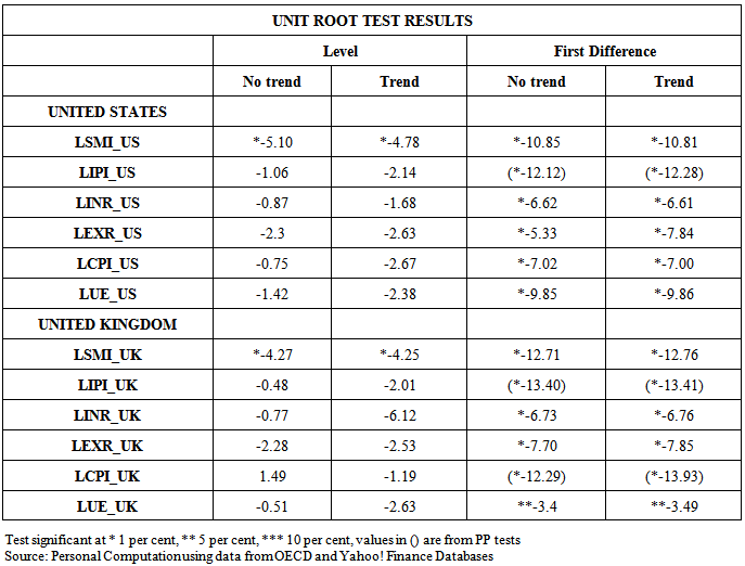
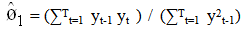
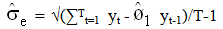
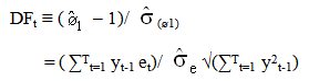
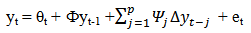
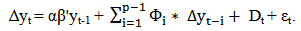
- The variables included in the analysis are short-term interest rates (INR), exchange rates (EXR), unemployment rates (UE), money supply M3, industrial production index (IPI) and consumer price index (CPI), the returns of FTSE100 (SMI_UK) and S&P500 (SMI_US). Money supply M3 served as exogenous variable in all the models to ascertain the effect of changes in government monetary policies. Also financial crisis was introduced as a dummy variable to capture structural breaks in the models especially due to the current global recession. All macroeconomic and stock returns variables were converted to log. Stock market returns were computed using the formula; yt= Log (yt/yt-1). Based on the time plots (appendix I and II), one can assume random walks for all endogenous and exogenous variables except the stock market returns, which seem to be stationary. The most frequently asked question in economic time series analysis is whether macroeconomic time series return to some long-run trend following a shock or whether they follow random walks. For example, if FTSE100 follows a random walk, the effects of a temporary shock such as increase in interest rates or drop in consumer price index will not dissolve after several months but instead will be permanent. If these variables do follow random walks, a regression of one against another can lead to spurious (non-sense) results because a random walk does not have a finite variance. Therefore Ordinary Least Squares (OLS) will not yield a consistent parameter estimator. Unit root tests – Augmented Dickey-Fuller (ADF) and Phillips Perron (PP) TestsTo check the stationarity of these series, this study carried out Augmented Dickey-Fuller (ADF) and Phillips-Perron (PP) unit root tests (Table 1.0) on the macroeconomic variables and the stock market returns. Dickey and Fuller (1979) postulated a test popularly referred to as the Dickey-Fuller test which uses a t-ratio test statistic. In summary, the test statistic is based on the least square (LS) estimate of the parameter ø1 in the simple models:
 | (1.1) |
 | (1.2) |
|
 | (1.3) |
 | (1.4) |
 | (1.5) |
 | (1.6) |
 – 1,
– 1,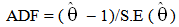 | (1.7) |
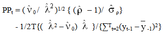
 is the LS estimates of θ (generally referred to as the Augmented Dickey-Fuller unit root test). Sometimes the result of a regular ADF test may indicate that a series is of higher order i.e. I(2) when infact it is I(1). An alternative unit root test developed by Phillips and Perron (1988) is flexible in dealing with serial correlation and heteroskedasticity in the error terms by ignoring any serial correlation that may be existent in the test regression. The test regression is
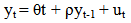 | (1.8) |
 | (1.9) |
 | (2.0) |
|
|
|
 | (2.1) |
 | (2.2) |
 | (2.3) |
 | (2.4) |
 | (2.5) |
|
 = -1.18 and
  = 0.79 are significant at 1 per cent. This is an indication that one can expect the LSMI_UK to converge to its long-run equilibrium at a fairly fast rate so as to allow the short-run dynamics. Specifically the adjustment will take about two and half months. For the equilibrium to be stable, it is necessary that a slight movement away from equilibrium position should set up forces tending to restore the equilibrium. Consequently, to uniquely determine the two cointegrating vectors, exchange rates and unemployment rates were removed from the first vector and restricted industrial production index to -1(additive inverse velocity relation5) in the second cointegrating vector by imposing restrictions on long-run coefficients
  (1,4)=0,
  (1,6)=0,
  (2,2)=-1. Furthermore, restrictions were placed on the speed of adjustments in the second, fourth, fifth and sixth error correction equations i.e
  (4,1)=0,
  (5,1)=0,
  (6,1)=0,
  (2,2)=0,
  (4,2)=0,
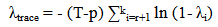
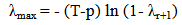
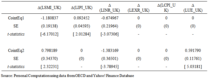
  (5,2)=0. The test of restrictions yielded a χ2 (6) value of 5.82 with p-value = 0.4429. This implies that exchange rate and consumer price index are weakly exogenous variables6. The normalized cointegrating vectors are as shown in Table 1.5 and Table 1.6. The VECM allows for the findings that the other endogenous variables Granger-Causes LSMI_UK or vice-versa as long as the error correction terms are statistically significant irrespective of the joint significance of the estimated coefficients (Aweda et al, 2014). In order to evaluate the long-run relations, we normalized first cointegrating vector on LSMI_UK. Surprisingly negative and significant relationship exists between stock market return and industrial production index. We also normalized the second cointegrating vector on industrial production index LIPI_UK and found a significant negative relationship with unemployment rates LUE_UK. Also, stock market return has a negative and significant relationship with industrial production index. A reason could be that this variable might not be the best proxy for measuring the real economy probably due to increased dependency on services innovation (tertiarisation). However, Sezgin et al. (2008) using GDP as the proxy for real output found significant negative short-run relationship between stock return of Istanbul Stock Exchange Index (ISE) and Turkey GDP. The positive relationship between interest rates and stock market return is in line with Fama (1981) who found strong positive correlation between common stock and real economic variable such as interest rates.
|
|
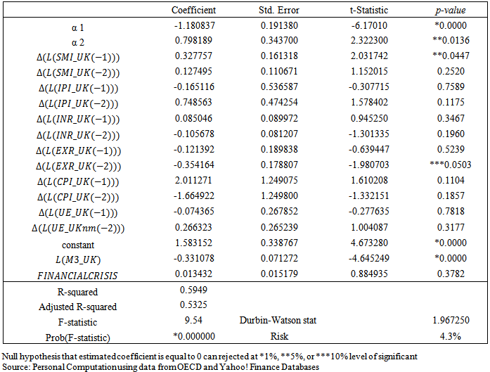
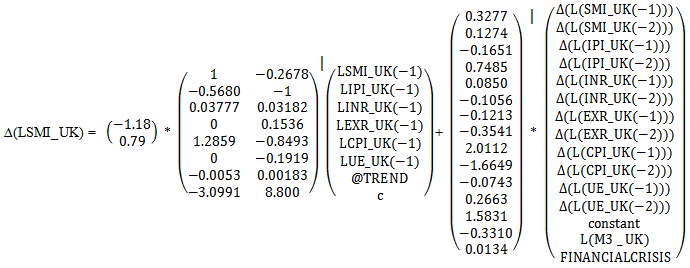 Residual Diagnostic Tests on FTSE100 Error Correction ModelA Durbin-Watson value of 1.96 indicates no serial correction in the VECM system error term and confirms long-run relationships that exist between the endogenous variables. One of the major problems associated with the Johansen test of cointegration is the insensitivity to the non-normality of residuals/innovations (Aweda et al, 2014). Therefore in order to ensure the avoidance of over-acceptance of cointegration, residual diagnostics were conducted for serial correlations, normality, ARCH7 (Autoregressive Conditional Heteroskedasticity) effect and Heteroskedasticity on the system equation
  . Jarcque-Berra value of 3.89 (p-value of 0.1429) indicates the residuals are multivariate normal Np (0, ∑), ARCH effect (n*R2 = 2.58, p-value = 0.2754) are insignificant at 10 per cent level. After conducting the Breusch-Godfrey Lagrange Multiplier test of serial correlation (n*R2 = 3.34, p-value = 0.1879) on the residuals one could not reject the null hypothesis of no serial correlation. The evaluation of the historical simulations or ex post forecasts using Theil inequality coefficient produced a value of 0.5788.Furthermore, covariance accounted for 72.47 per cent, variance 27.52 per cent while bias proportion is 5.6x10⁻⁵ per cent. Usually the best model has a Theil Inequality value close to zero and the covariance portion very high (> 60 per cent) indicating a strong correlation between the actual and forecasted values. Forecast errors reflect external shocks on the VECM model. These errors are mostly episodic in nature such as highlighted below. Others are completely chance variations which are completely isolated. In the case of LSMI_UK, these shocks were observed in:
  August and September 2002 - speculation over the invasion of Iraq.
  December 2007 to November 2010 - tight market liquidity.
  August and September 2008 - global financial crisis, collapse of Lehmann Brothers, Bank of America agreed to purchase investment bank Merrill Lynch, and insurance giant AIG sought an abridged loan from Federal Reserve Bank of America and the biggest bank failure in history occurred when JP Morgan Chase agreed to purchase the banking assets of Washington Mutual. Northern rock was nationalised after unsuccessful take-over bids.
  December 2009 - increased activities in the properties sector; house prices rose by 2.9 per cent.
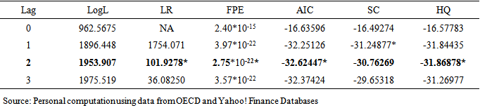
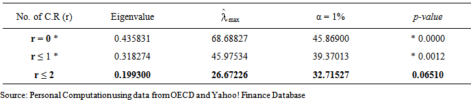
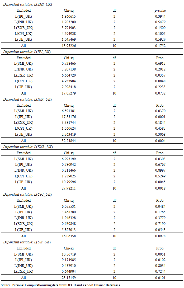
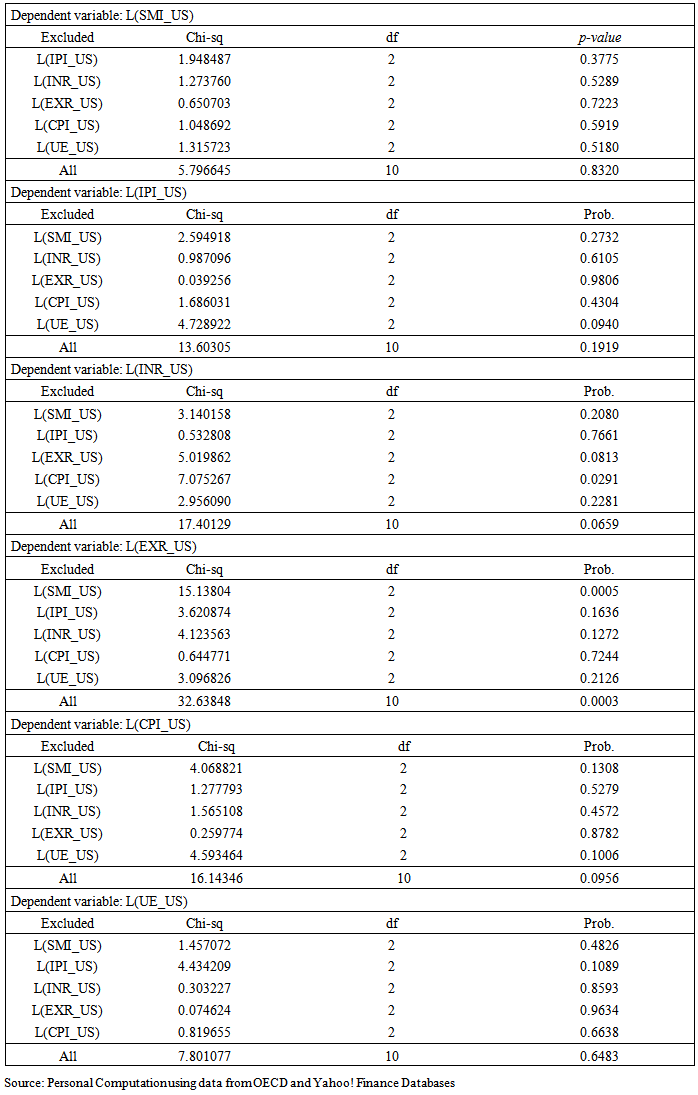
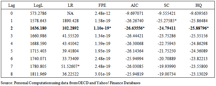
 July 2011 to April 2012 - persistent sovereign debt crisis in the euro zone.Relations between S&P500 Stock Market Return and Macroeconomic VariablesTest of Granger non-causality among the variables indicate reasonable evidence of causal relationships amongst them (appendix IV). A unidirectional causal relationship exists from stock market return to exchange rates and not vice versa. Similarly, a unidirectional causal relationship exists between consumer price index and exchange rate to interest rates but not vice versa. In the case of the remaining endogenous variables the reason for some granger non-causality could be that the sample sizes are insufficient to satisfy the asymptotic conditions that the cointegration and causality tests rely on. These causal relationships indicate there could be long run relationships amongst the variables. Therefore, a further test of cointegration was carried out using two lags which was selected based on the results of lag order selection (see table 1.8).
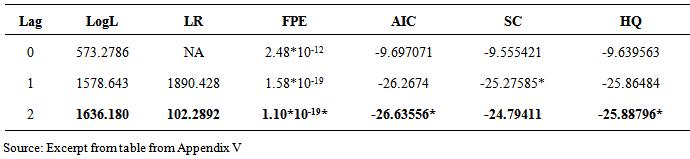
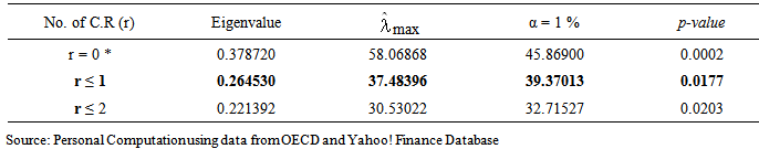
|
|
 (1,1)=1,
  (1,2)=0,
  (2,1)=
  (3,1)=
  (5,1)=
  (6,1)=0. The restriction test yielded a χ2 (5) value of 6.34 (p-value = 0.2745). Hence, industrial production index, short-term interest rate, consumer price index and unemployment rate were reconsidered to be weakly exogenous in this model. The cointegrating vectors are as shown in table 2.0 and Table 2.1 below.
 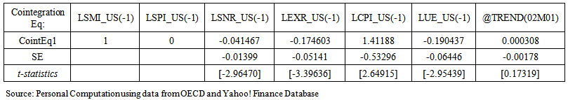 | Table 2. Restricted Normalized Cointegrating Equation-S&P500 VECM |
|
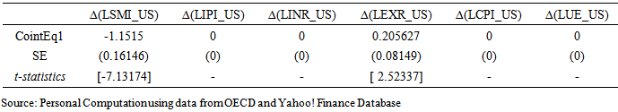
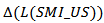 indicates that though the model is highly significant at 1 per cent level with F-value = 8.63 and p-value = 0, the endogenous variables accounted for more than 54 per cent of the total variation in LSMI_US. The Durbin-Watson value of 1.97 lies within the interval 2 < DW< 4-du, where du = 1.65 is the upper limit of the Durbin Watson table of critical values at 1 per cent level of significance. This signifies the co-movement of the endogenous variables in the long-run. The Vector Error Correction Model system equation is as shown in the equation below:
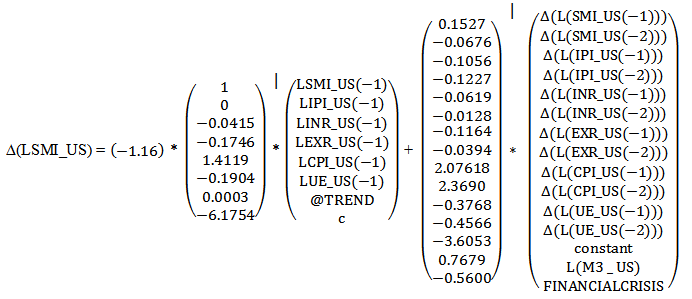
|
 May, August and September 2002 - speculations over invasion of Iraq.
 February to April 2005 - market volatility in the Euro zone.
 October and December 2007 - US growing debt and housing bubble, rising foreclosures. Car sales were down by 2.4 per cent which was a strong indication of looming recession.
 May 2008- there was strong liquidity crisis as a result of anticipation of recession in addition to high energy prices.
 September 2008 - Lehmann Brothers declared bankruptcy.
 January 2009 - rising unemployment rates.
 August 2011 - US lost its coveted AAA credit rating by Standard & Poor, European debt crisis continue to persist. There was also rising fear of a new US recession (GDP dropped to 1.3 per cent in Q1 2011 from 2.5 per cent in 2010 second time in a row).
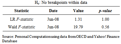
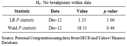
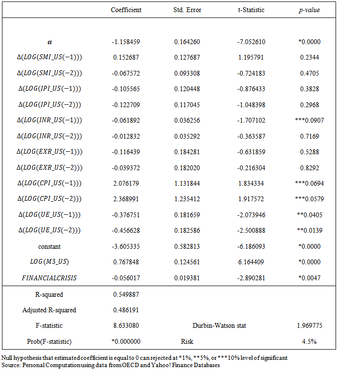
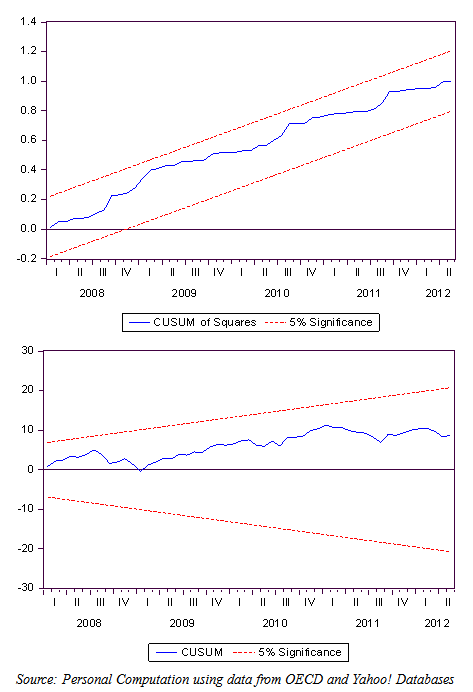
 April 2012 - Sovereign debt crisis in the euro zone persists.Models Stability DiagnosticsThe CUSUM and CUSUM of square tests as suggested by Brown et al. (1975) were employed to evaluate the cumulative sum of recursive residuals. The formal employs the test statistic Vt = ∑tp=k+1 vp/σv to ascertain parameter instability arising from cumulative sum falling outside areas between [k, ± -0.948(T-k)1/2] and [T, ± 3*0.948(T-k)1/2] of 5 per cent critical areas. The range is dependent on time t. The E(Vt) = 0 if the vector of parameters β remains regular. The CUSUM square test on the other hand is based on calculating the test statistics Sp = (∑tp=k+1v2p)/ (∑Tp=k+1v2p) with an expected value E(Sp) = (t-k)/ (T-k) which takes value zero if t = k and 1 if t = T under parameter constancy. Refer to Brown et al (1975) for details of table of significance lines for CUSUM of squares test. The necessary condition for recursive tests is that the disturbances or residuals must be multivariate normally distributed (Brown et al., 1975). The stability check carried out on the two models using graphical examination of recursive tests are displayed in Figure 3 and 4. It can be seen that there is little evidence of structural instability in the estimated model. Likewise, the cumulative sum of forecast errors does not cross the 5% critical lines in the recursive tests and, consequently, the null hypothesis of model stability cannot be rejected.
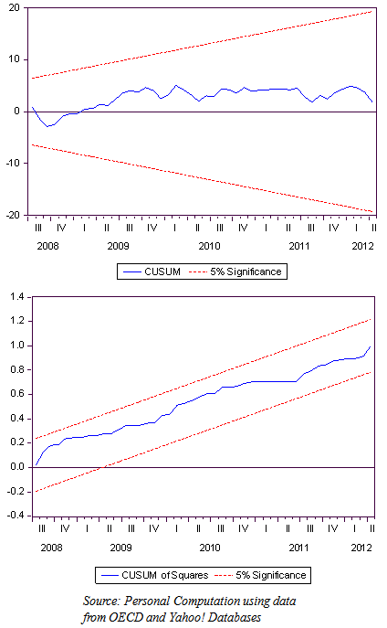 | Figure 3. CUSUM and CUSUM Square Plots for returns on FTSE100 |
 | Figure 4. CUSUM and CUSUM Square Plots for returns on S&P500 |
3. Conclusions and Economic Implications of Results
- Sequel to the dynamic rate of stock market returns common to the two markets analysed in this research work, one can conclude that the efficient market hypothesis is essentially valid in the sense that the monthly rate of returns are stationary over pre- and post-financial crisis periods. Although the average rate of return in S&P500 is marginally higher than the FTSE100, the relative risk of return of 4.5 per cent in US is higher than UK (4.3 per cent). For the entire period, the global test of the combined effects of all the endogenous and exogenous variables in each market turned out to be significant in forecasting the respective stock market returns. More than 50 per cent of the total variation in stock market returns was accounted for by all the endogenous and exogenous variables in each market. Long-run co-movement amongst the endogenous variables was established in each of the market though with varying speed of adjustment from disequilibrium caused by shocks on the stock market returns. The adjustment to equilibrium in the long-run is expected to take about one month in the United States and 2.5 months in the United Kingdom so as to allow short-run dynamics. The slower speed of adjustment to equilibrium in the United Kingdom was attributable to the additive inverse velocity relationship between industrial production and the return on FTSE100. In the FTSE100 model, the stock market return depended in the long-run on industrial production index, interest rates and consumer price index while relationship existed between stock market return, exchange rates and unemployment rates only through industrial production index. On the other hand, return on S&P500 was influenced in the long-run by interest rates, exchange rates, unemployment rates and consumer price index (CPI). However, increase in industrial production index resulted in a rather surprising decline in stock market return in UK in the long-run. The industrial production lags general economic activity. As a result of this negative relationship, industrial production index was considered inappropriate proxy for measuring real economic activities in the UK, which may be linked to the fast service innovations or tertiarisation of the economy.The short-run dynamics reveal exchange rates, consumer price index are significant in United Kingdom. However, industrial production index, interest rates and unemployment rates have no significant short-run relationships with return on FTSE100. Similarly, industrial production index in addition to exchange rates have no significant short-run causality with S&P500, which is rather surprising. In both markets the economic theory plays a much stronger role in determining the models’ long-run properties than the short-run dynamics, which is largely data-determined. Whilst increase in BoE monetary policy measured by broad money supply M3 lead to a significant decline in the stock market return on FTSE100, the return on S&P500 increased significantly due to the intervention of Federal Reserve. This was largely due to increased inflation in the short-run in United Kingdom and excess liquidity in the United States which is a direct impact of series of quantitative easing QE programmes especially QE2 in 2010 by the Federal Reserve. QE2 had a significant positive impact on industrial production or output through lower interest rates, which translated into higher stock prices in the long-run. Other factor associated with this was the fact that United States profits from the capital flights from European countries as a result of the persistent sovereign debt crisis. The impact of the 2007 – 2012 global financial crises was evaluated in each of the market. Although the effect of this dummy variable was negative and significant in the US signalling potentially insecure financial system, the crisis was positive but statistically insignificant in United Kingdom probably due to stable fiscal policy and other structural issues such as spending cuts, budget deficit reduction and housing policies adopted by the government. This further explains the higher risk of investing in the United States. This exogenous variable was introduced to evaluate the effect of inherent structural breaks in the markets. Analysis of forecast error signified the impact of important shocks from external forces on stock market returns. The speculation about Iraq war of 2002 was observed in the two models, which lead to significant drop in returns at start of the war but stabilized during the war. Also the global financial crisis, which began in November of 2007, was revealed in the forecast errors of the models. Similarly, current financial crisis in the Euro zone was also accounted for in the forecast errors. However, each market has peculiar shocks from external forces distorting the forecast errors at various points. These include but not limited to tight market liquidity caused by the collapse of many banks resulting in significant outflows of cross-border interbank deposits, increased activities in the property sector in the United Kingdom, US losing its AAA credit rating by Standard & Poor and lingering sovereign debt crisis in the euro zone. There was also rising fear of a new US recession after the GDP dropped two quarters in a row between 2010 and 2011. Stock market return on S&P500 reacts quicker to shocks on macroeconomic variables, which were also reflected in the speed of adjustment to equilibrium in the long run. While the effect of unemployment rates will be negative on FTSE100, it is expected to have rather surprising positive effects on the S&P500 stock market index. The steady drop in unemployment rate since 2012, largely attributable to QE3 introduced by the Federal Reserve in September 2012 in continuation of its unconventional monetary policy was expected to have positive impact on overall output and keep inflation rate below 2 per cent target. This in turn is good news for stock prices and returns. Conversely, the rising inflation rate is an indication of imminent economic instability particularly in the United Kingdom. Above-target inflation rates will continue to have negative effects on the exchange rates, which in turn may result in fall in output in the short- to medium-term in United Kingdom. Therefore, interest rates may have to be increased in the future to check the growth of inflation rate which can have positive effects on aggregate output. In conclusion, this research work has shown that stock market returns are important leading economic indicators for predicting the direction of economic activities in both United Kingdom and United States. Hence, the presence of a well-specified and stable relationship between stock market returns and macroeconomic variables can be seen as imperative for investors’ confidence and sustainable long-term economic growth. Stability can be achieved by efficiently controlling changes in these macroeconomic fundamentals, which limit the variations of the economy without preventing it from fluctuating in general. Also, a stable monetary policy (either conventional or unconventional) is not enough. It can be complemented by a secure fiscal policy through the tax system or efficient government spending which affects aggregate expenditure rapidly and directly will change the level of employment and output without necessarily resulting in high inflation.
Appendix I
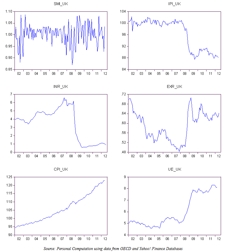 | Figure 1. Time Plots on FTSE100 stock returns and Macroeconomic variables |
Appendix II
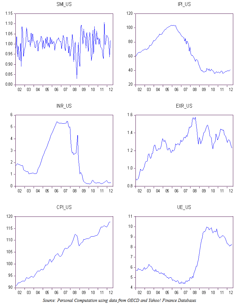 | Figure 2. Time Plots on S&P500 stock returns and Macroeconomic variables |
Appendix III
Appendix IV
Appendix V
Notes
- 1. QE also called large-scale assets purchases (LSAPS) are effective alternative to conventional monetary policy when interest rates are close to zero2. Countercyclical economic indicators have an inverse movement with the economy i.e unemployment rates tends to get larger as the economy changes from expansion to recessionary business cycle.3. Quandt-Andrews breakpoint test is a modified version of Chow Test that uses Likelihood Ratio Test. QA breakpoint test follows a non-standard distribution and it automatically computes the usual Chow F-test repeatedly with differing break dates. The Break date with the largest F-statistic is chosen. 4. A parameter is nuisance parameter if its value influences the distribution of observations even though one is not interested in its values.5. AIVR is a negative relationship between industrial production index and stock market return on FTSE 100 resulting in the opposite directional speed adjustment to long-run equilibrium.6. The parameters of weakly exogenous variables have marginal density function bearing no relation to the parameters that determine the conditional density function of a dependent variable.7. ARCH assumes that all pairwise autocorrelations are zero. In stock market returns large and small errors tends to occur in clusters hence according to Engle, the recent past gives information about the conditional disturbance variance σ2t .