Avuglah R. K. , Adu-Poku K. A. , Harris E.
Department of Mathematics, Kwame Nkrumah University of Science and Technology Kumasi, Ghana
Correspondence to: Adu-Poku K. A. , Department of Mathematics, Kwame Nkrumah University of Science and Technology Kumasi, Ghana.
| Email: |  |
Copyright © 2014 Scientific & Academic Publishing. All Rights Reserved.
Abstract
Road traffic accident cases in Ghana are increasing at a fast rate and this has raised major concerns. The World Health Organization (WHO, 2001) report indicates that about 50 million people are injured on the roads and 1.2 million people are killed each year. This paper applies the Autoregressive Integrated Moving Average (ARIMA) time series model to study the trends and patterns of road traffic accident cases in Ghana as well as makes a five- year forecast. An Annual accident data from 1991 to 2011 was obtained from the National Road Safety Commission and the Building and Road Research Institute in Ghana. The results showed that road traffic accident cases are increasing in Ghana. Models were subsequently developed for accident cases and ARIMA (0,2,1) was identified as the best model. A Five- year forecast was made using the best model and it showed that road traffic accident cases would continue to increase in Ghana.
Keywords:
Autoregressive (AR), Moving average (MA) and ARIMA
Cite this paper: Avuglah R. K. , Adu-Poku K. A. , Harris E. , Application of ARIMA Models to Road Traffic Accident Cases in Ghana, International Journal of Statistics and Applications, Vol. 4 No. 5, 2014, pp. 233-239. doi: 10.5923/j.statistics.20140405.03.
1. Introduction
Research has indicated that Road Traffic Accidents are a leading cause of injury and death around the world and a major public health problem (Penden et al., 2004). About 50 million people are injured and 1.2 million people are killed each year in road crashes worldwide (Penden et al., 2004). Reports from the World Health Organization strategy of 2001 indicates that presently road traffic accidents are the leading cause of deaths and the 9th leading contributor to the burden of disease Worldwide based on disability adjusted life years (WHO, 2001).In Ghana, there has been a simultaneous increase in the number of vehicles on roads with increased road safety campaign and unfortunately, road conditions, vehicle maintenance and driver instructions have not grown accordingly.At least 1,800 deaths are recorded every year and 6 people die every day as a result of road traffic crashes in Ghana (NRSC, 2013). Moreover, 60% of victims involved in road traffic accident are aged 15 and 55 years (NRSC, 2013). Statistics from the National Road Safety Commission in Ghana indicates that from the period of 2001 to 2011, 125,657 crashes of road traffic accident have been recorded resulting to 21,267 deaths (NRSC, 2012).Road accidents are known to be associated with driver error, vehicle conditions, road environment, over speeding, road users and a variety of factors (Aworemi et al., 2010). Research has shown that human factors (pedestrians) account for about 90% of all causes of road accidents in New York (Shinar, 1978). The situation is not different in Ghana as statistics indicate that pedestrian’s death remains the leading cause of fatality among urban road users. (Afukaar et al., 2003). Similar research indicates that pedestrians constitute about 43% of the total road traffic fatalities most of whom fall within the active age group of 16-45 years (Afukaar et al., 2003). Over speeding has also been found to be one of the most common contributory factors in vehicle crashes (Afukaar et al., 2003). Much work on road accident has been done within the context of regression analysis. A recent study employed binary and multinomial logit regression models to study the effect of posted speed limits on road accidents and found that speed limits do not have any significant effect on road accident (Nataliya, 2006). Kweon and Kockeleman (2003) used Poisson and ordered probit model to analyze road accident and found that young drivers are far more crash prone than older drivers. Logistic regression model was used by (Macleod et al., 2011) to analyze hit and run accident cases in USA. Road traffic accident research has extensively been considered within the framework of time series analysis. In Nigeria, time series research has shown that road traffic accidents are on the decrease with the exception of Lagos Island local Government area (Atubi et al., 2013). Similarly, predicted results from ARIMA time series model revealed that road traffic accident cases are going to increase from 107,579 to 401,536 over the next one year in China (Yuan-Yuan Pack et al., 2013). ARIMA model was used in predicting Malaysian road fatalities for the year 2015 and 2020 and the results showed that the predicted fatalities for the year 2015 will be 8,760 and 10,716 in 2020 (Rohayu Sarani et al., 2012). It is in this direction that this paper is prepared to study the trends, patterns and forecast of road traffic accidents in Ghana.
2. Materials and Methods
2.1. Data
Data for the study was secondary, a historical annual traffic crash data for the years 1991 through to 2011 compiled by the National Road Safety Commission and Building and Road Research Institute in Ghana. The analysis was computationally implemented in the R software.
2.2. Model Specification, Estimation and Test
ARIMA is the method introduced by Box and Jenkins. This method of forecasting implements knowledge of autocorrelation analysis based on Autoregressive integrated moving average models. The method is of four distinct stages namely Identification, Estimation, Diagnostics checking and Forecasting.
2.3. Stationarity
A time series is stationary if there is no systematic change in mean (no trend), variances and strictly periodic variations have been removed. In other words, when the value of time origin, n is increased, the change will have no effect on the joint distribution which must depend on the interval. Mathematically, a time series is said to be stationary if the joint probability distribution of  is the same as the joint distribution of
  for all
  .Alternatively, a time series is said to be stationary if:
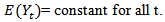 | (1) |
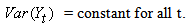 | (2) |
 | (3) |
2.4. Achieving Stationarity
Due to the non-stationary nature of most business and economic time series, it is required that stationarity be achieved before building any model.We can difference the data.The differenced data will contain one less point than the original.For non-Constance variance, taking the logarithm or square root will stabilize the variance.For non seasonal data, first order differencing is usually sufficient to attain apparent stationarity so that the new series  is formed from the original series
  by
by  Occasionally, second order differencing is required using the operator
  where
where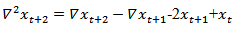 | (4) |
Hence the number of times that the original series is differenced to achieve stationarity is the order of homogeneity.
2.5. Differencing
This is a special type of filtering which is particularly useful moving a trend. This is achieved by subtracting each data in a series from its predecessor. For non-seasonal data, first order differencing is sufficient to obtain apparent stationarity. The concept of backshift operator helps to understand and express differenced ARIMA models. For example,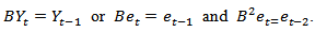 | (5) |
ARIMA (1,0,0) can be expressed in terms of backshift operator as | (6) |
 but
but  put into equation (6), we get
  | (7) |
Similarly, ARIMA (2,0,0) can be written as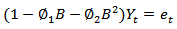 | (8) |
 | (9) |
2.6. ARIMA (p, d, q) Models
If an observed time series is non-stationary in the mean, then we can difference the series. If Yt is replaced by  in the equation
 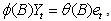 then we have a model capable of describing certain types of non-stationary series. Such a model is called an integrated model.The general ARIMA (p,d,q) is of the form:
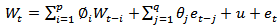 | (10) |
And p is the order of the AR part, d is the degree of differencing and q is the order of the MA part. An example of ARIMA (p,d,q) is ARIMA (1,1,1) which has one Autoregressive parameter, one level of differencing and one Moving average parameter is given by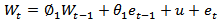 | (11) |
 | (12) |
Examples of ARIMA models are as ff: | (13) |
 | (14) |
 | (15) |
 | (16) |
 | (17) |
2.7. Box and Jenkins Method
This method of forecasting implements knowledge of autocorrelation analysis based on autoregressive integrated moving average models. The procedure is of four main stages namely:IdentificationEstimationDiagnostics CheckingForecasting
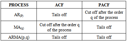
2.8. Identification
The first step in developing an ARIMA model is to determine if the series is stationary. If the model is found to be non-stationary, stationarity could be achieved mostly by differencing the series or going for the dickey fuller test. Stationarity could also be achieved by some mode of transformation like the log transformation. Once stationarity has been achieved, the next step is to determine the orders of the autoregressive (AR) and moving average (MA) terms using the Auto Correlation Function (ACF) and Partial Auto Correlation Function (PACF). The table below shows how p and q orders of ARIMA models are identified.Table 1. Identification of p and q orders in ARIMA Models
 |
| |
|
2.9. Estimation
Once the preliminary model is chosen, the estimation stage begins. The purpose of estimation is to find the parameter estimates that minimize the mean square error. Two approaches are used and these include the nonlinear least squares and maximum likelihood estimates. In this method, the R statistical package was used in the estimation.
2.10. Diagnostics Checking
Residuals from the model are examined to ensure that the model is adequate (random). The following diagnostics are made:Time plot of the residualsPlot of the residual ACFNormal Quantile Quantile (QQ) Plot
2.11. Forecasting
When a satisfactory ARIMA model has been found to be adequate, then we proceed to forecast or predict for a period or several periods ahead. However, chances of forecast errors are inevitable as the period advances.
3. Analysis and Results
3.1. Preliminary Analysis
Figure 1 shows the time plot of accident cases in Ghana from 1991-2011. The time plot exhibits a systematic change, therefore giving evidence of trend in the data. Accident cases in Ghana decreased from 1991 to 1994 but increased sharply from 1995 to 1998. An irregular and inconsistent pattern was observed from 2000 to 2011. The accident data are not stationary and do not exhibit seasonal variation. Minimum peak of 6467 accident cases occurred in 1993. In 2009, a maximum peak of accident cases were recorded which amounted to 12299.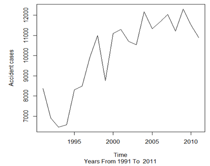 | Figure 1. Time plot of accident cases in Ghana from 1991 to 2011 |
The plots exhibit a moving trend hence there is the need to apply differencing to achieve stationarity.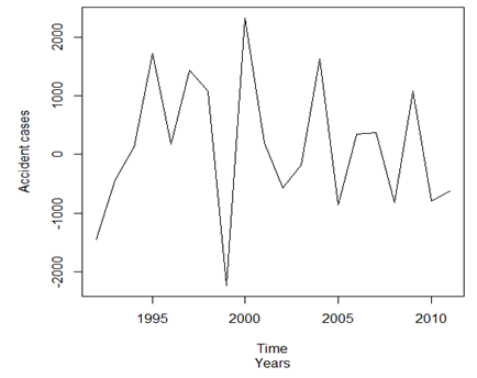 | Figure 2. First differencing of accident cases in Ghana |
First differencing was performed to remove trend component in the original data.
3.3. Second Differencing of Accident Cases in Ghana
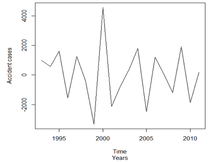 | Figure 3. Second differencing of accident cases in Ghana |
Second differencing was done to achieve better stationarity. The variability was approximately constant and the accident data appears to be approximately stable.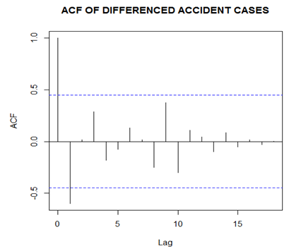 | Figure 4. ACF plots of the second differencing of accident cases in Ghana |
From Figure 4, only lag 1 is significant implying a moving average of order 1 (MA 1).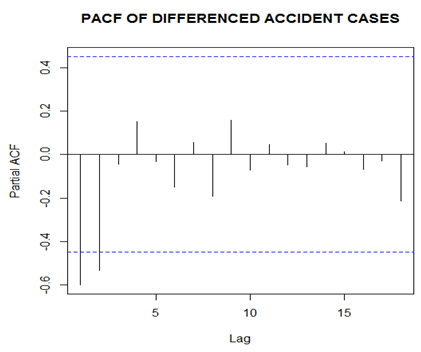 | Figure 5. PACF plots of the second differencing of accident cases in Ghana |
From Figure 5, comparing the partial Autocorrelation function with the error limits, we choose AR (2).The following models were suggested; ARIMA (2,2,1) ARIMA (2,2,0)ARIMA (0,2,1)Selection of the best model was examined with respect to the diagnostics of residuals, parameter estimates, Akaike Information Criterion (AIC), Akaike Information Criterion Corrected (AICC) and Bayesian Information Criterion values.
3.4. Parameter Estimation
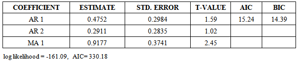
The t-value for MA 1 is statistically significant while that of AR 1 and AR 2 are not statistically significant since the t-value is less than 2 in absolute terms (Table 2).Table 2. ARIMA (2,2,1) MODEL
 |
| |
|
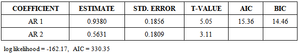
From Table 3, the parameter based on the t-value test is statistically significant.Table 3. ARIMA (2,2,0) MODEL
 |
| |
|
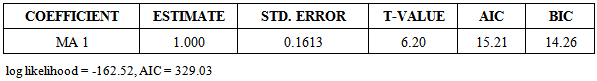
From Table 4, the parameter based on the t-value test is statistically significant.Table 4. ARIMA (0,2,1) MODEL
 |
| |
|
3.5. Model Diagnostics
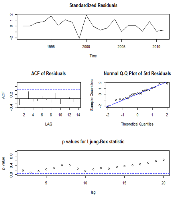 | Figure 6. Diagnostics of the residuals from ARIMA (0, 2, 1) |
Diagnostics of the residuals from ARIMA (0, 2, 1) is shown in the Figure 6 above. The standardized residuals plot shows no obvious trend and pattern and looks like an independent and identical distribution. The plot of the ACF of the residuals of the diagnostics shows no evidence of significant correlation in the residuals. Most of the residuals are located on the straight line except some few outliers deviating from the normality and lastly the bottom part of the diagnostics was the time plot of the Ljung- Box statistics plot which was not significant at any positive lag. In conclusion, the model is adequate and fits well.It is also observed that ARIMA (2,2,1) and (2,2,0) models exhibited similar diagnostics characteristics as ARIMA (0,2,1).
3.6. Selection of Best Model for Forecasting Accident cases in Ghana
The standardized residuals plots of all the models were independently and identically distributed with mean zero and some few outliers. There was no evidence of significance in the autocorrelation functions of the residuals of all the models and the residuals appear to be normally distributed in all the models. The Ljung – Box statistics is not significant at any positive lag for all the models. From Table 2-4, the parameters of ARIMA(2,2,0) and ARIMA(0,2,1) models are significant except ARIMA (2,2,1). The AIC, BIC and residual variance are good for all the models but favored ARIMA (0,2,1) model. Since ARIMA (2,2,1) is not significant, the parameters of ARIMA (2,2,0) and ARIMA (0,2,1) are compared.Comparing the AIC of the models, we could observe that ARIMA (0,2,1) had the minimum AIC and residual variance.From the discussion above, it is evident that ARIMA (0,2,1) is the best model for forecasting accident cases in Ghana. This therefore leads to the use of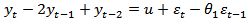 | (18) |
Where 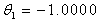 The fitted ARIMA (0, 2, 1) model for forecasting accident cases from 1991-2011 is given by
 | (19) |
Table 5. Forecasting accident cases in Ghana
 |
| |
|
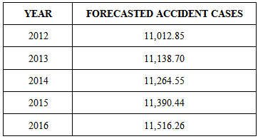
Figure 7 gives the visual representation of the accident cases data (black line), its forecasts (red line) and confidence interval (blue short dashes lines). | Figure 7. Graph of the accident cases, its forecast and confidence intervals |
From the prediction values and the graph above, it can be observed that, accident cases in Ghana will continue to increase in the next 5 years.
4. Conclusions
Time series analysis of the data from the years 1991 – 2011 showed that the patterns of Road Traffic Accident cases are increasing in Ghana. ARIMA (0,2,1) is identified to be the suitable model for the road accident data. Predictions from ARIMA (0,2,1) model revealed that road traffic accident cases in Ghana will continue to increase over the next 5 years. The findings of this study draw attention to the importance of implementing key road safety measures in order to change the increasing pattern of road accident in Ghana. Therefore, improved and better policies of National road safety commission should be introduced with much emphasis on publication and education to ensure maximum reduction in Road accident crashes.
References
| [1] | Afukaar, F.K., Antwi, P., and Ofosu-Amaah, S. (2003). Pattern of road traffic injuries in Ghana: implications for control. Injury control and safety promotion.vol. 10 (No. 1-2):69-76. [PubMed: 12772488]. |
| [2] | Afukaar, F.K., Antwi, P., and Ofosu-Amaah, S. (2003). Speed control in developing countries: issues, challenges and opportunities in reducing road traffic injuries. Injury control and safety promotion; Vol. 10 (No. 1-2): 77-81. [PubMed 12772489]. |
| [3] | Atubi, A.O. (2013). Time series and trend analysis of fatalities from road traffic accident in Lagos State, Nigeria. Mediterranean journal of social sciences, vol.4 (1) January 2013. Doi: 10.5901/mjss.2013.V4n1p251. ISSN:2039-9340 |
| [4] | Aworemi, J.R., Abdul-Azeez, I.A., and Olabode, S.O. (2010). Analytical studies of the causal factors of road traffic crashes in South Western Nigeria. International research journals. Educational research Vol. 1(4)pp. 118-124. www.interesjournals.org/ER. |
| [5] | Kweon, Y.J., and Kockelman, K. M. (2003). Overall injury risk to different drivers: combining exposure, frequency, and severity models. Accident Analysis and Prevention, 35, 441 |
| [6] | MacLeod, K.E., Julia, B., Griswold, L.S., and Arnold, D.R. (2011). Factors Associated with Hit-and-Run Pedestrian Fatalities and Driver Identification. Accident Analysis and Prevention 45(2012) 366-372. www.elsevier.com/locate/aap. |
| [7] | Nataliya, V.M. (2006). Influence of posted speed limit on roadway safety. Accident Analysis and Prevention, 33, 569. |
| [8] | National Road Safety Commission (NRSC, 2013). “4th National Road Safety Awards”.(www.nrsc.gov.gh/site/news/34). |
| [9] | National Road Safety Commission (NRSC, 2012). Press release Dec, 2012 (www.nrsc.gov.gh/site/news/16). |
| [10] | National Road Safety Commission (NRSC, 2012) Ghana’s response to the road safety challenge. The road between US-ACCRA. (info@nrsc.gov.gh, www.nrsc.gov.gh). |
| [11] | Peden, M. (2004). World Report on Road Traffic Injury Prevention. World Health Organization, Geneva. |
| [12] | Rohayu, S., Sharifah Allyana, S.M.R., Jamilah, M.M., and Wong, S.V. (2012). Predicting Malaysian road fatalities for year 2020. Kuala Lumpur: Malaysian Institute of Road Safety Research 2020, MRR(6)2012. |
| [13] | Shinar, D. (1978). Psychology on the road: The human factor in traffic safety, New York, John Wiley and Sons. ISBN: 9780471039976. |
| [14] | World Health Organization, (2001). Global Pollution and Health Related Environmental Monitoring, London, U.K. |
| [15] | Yuan,Y.P., Xu-jun, Z., Zhi-bin, T., Meng-jing, C., and Yue, G. (2013). “Autoregressive Integrated Moving Average Model in predicting road traffic injury in China”. Zhonghua Liu Xing Bing Xue Za Zhi 2013 Jul; 34(7):736-9. |
 Abstract
 Reference
 Full-Text PDF
 Full-text HTML