Victor Mooto Nawa
Department of Mathematics and Statistics, University of Zambia, P.O. Box 32379, Lusaka, Zambia
Correspondence to: Victor Mooto Nawa, Department of Mathematics and Statistics, University of Zambia, P.O. Box 32379, Lusaka, Zambia.
| Email: |  |
Copyright © 2014 Scientific & Academic Publishing. All Rights Reserved.
Abstract
An alternative method of estimating parameters in a mixture model for longitudinal trajectories using the expectation – maximization (EM) algorithm is proposed. Explicit expressions for the expectation and maximization steps required in the parameter estimation of group parameters and mixing proportions are derived. Expressions for the variances of group parameters and mixing proportions for the mixture model are also derived. Simulation results suggest that results from the proposed approach are less dependent on starting values and therefore a good alternative to the current approach which is based on the Quasi-Newton method.
Keywords:
Mixture model, Longitudinal trajectory, PROC TRAJ, Quasi-Newton, EM Algorithm
Cite this paper: Victor Mooto Nawa, A Mixture Model for Longitudinal Trajectories, International Journal of Statistics and Applications, Vol. 4 No. 4, 2014, pp. 181-191. doi: 10.5923/j.statistics.20140404.02.
1. Introduction
Mixture models have been used extensively in a variety of important practical applications. In a mixture model, data can be viewed as arising from two or more populations mixed in varying proportions. There is a close link between clustering and finite mixture models. Cluster analysis is the search of groups of related observations in a data set. For example, in taxonomy clustering is used to identify subclasses of species. Fraley and Raftery (2002), outline a general methodology for model-based clustering. A number of researchers have studied finite mixture models in the context of clustering. In finite mixture models, each component probability distribution corresponds to a cluster. McLachlan and Basford (1988), highlighted the role of finite mixture distributions in modelling heterogeneous data, with the focus on applications in the field of cluster analysis. Their main focus was on mixtures of normal distributions. The problem of estimating parameters in a normal mixture distribution was first considered by Pearson (1894). Other researchers who have studied mixtures of normal distributions include Day (1969), Wolfe (1970), Marriot (1975) and Symons (1981). Mixtures of other distributions that have been considered by other researchers include exponential (Rider, 1961), beta (Bremmer, 1978), Weibull (Kao, 1959) and binomial (Blischke, 1962, 1964; Rider, 1962).Most researchers have concentrated on the fitting of mixture models by a likelihood based approach using maximum likelihood estimation with the EM algorithm providing a convenient way for the iterative computation of solutions of the likelihood equation (Redner, et al, 1984; Biernacki, et al, 2003; O’Hagan, et. al, 2012). However, other methods that have been used include method of moments, minimum chi-square, least squares and Bayesian methods. Day (1969), showed that the method of moments, minimum chi-square and Bayesian methods are inferior to the maximum likelihood method.Under the mixture likelihood approach to clustering, it is assumed that the observations to be clustered are from a mixture of an initially specified number of populations or groups mixed in various proportions. This approach to clustering is model based in the sense that the form of the density of an observation in each of the underlying populations is specified. One advantage of model based clustering is that it provides a specific framework for assessing the resulting partitions of the data and especially for choosing a relevant number of clusters (Biernacki, et al, 2000). By assuming some parametric form for the density function in each of the underlying groups, a likelihood is formed in terms of the mixture density and unknown parameters are estimated by maximum likelihood estimation. A probabilistic clustering of the observations is obtained in terms of their estimated probabilities of group membership. The assignment of the observations to the groups is done by allocating each observation to the group to which it has the highest probability of belonging.In this paper we present a mixture of developmental trajectories. Our focus will be on the semiparametric group based model proposed by Nagin (1999). The model assumes that the population is composed of a mixture of distinct groups defined by their developmental trajectories. This model is designed to identify rather than assume distinctive groups of trajectories, estimate the proportion of the population following each trajectory, relate group membership to individual characteristics and create profiles of group members using group membership probabilities (Nagin, 1999). The model presumes that two types of variables have been measured: response variable and covariates or risk factors.Jones, Nagin and Roeder (2001), wrote a SAS based procedure that can be used to estimate the parameters of this semiparametric model. The parameters are obtained by maximum likelihood estimation using the general Quasi-Newton procedure. Standard errors are obtained by inverting the observed information matrix. This software is a customized SAS procedure that was developed with the SAS product SAS/TOOLKIT. The SAS procedure is called is called PROC TRAJ.Whereas, the semiparametric model can be used to model three data types – count, binary and psychometric scale data, we will concentrate on binary data. Roeder et al. (1999) concentrated on count data using the EM algorithm. This paper will concentrate on binary longitudinal data using the EM algorithm. While Roeder et al. (1999) looked at a model that incorporated covariates, this paper will concentrate on a model without covariates.The remainder of this paper is organised as follows. The model under discussion is presented in Section 2. This section begins with a discussion of the standard mixture model in Section 2.1. The longitudinal mixture model, which is the main subject of this paper, is presented in Section 2.2. Section 2.2.1 gives the likelihood formulation of the longitudinal mixture model and the E-steps and M-steps required to estimate the group parameters as well as the mixing proportions in the model. This is followed by a discussion on estimation of standard errors for the group parameters and mixing proportions in Section 2.2.2. Simulation results are presented in Section 3 and conclusions are presented in Section 4.
2. The Model
2.1. Standard Mixture Model
A standard g-component mixture model (McLachlan and Basford, 1988) takes the form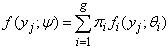 | (1) |
where yj is an observation on a random variable Yj and ψ = (θ1, θ2, …, θg, π1, π2, …, πg-1) is a vector of all unknown parameters. The underlying population is modelled as consisting of g distinct groups C1, C2, …, Cg in some unknown proportions π1, π2, …, πg and where the conditional function of Yj given membership of the ith group Ci is fi(yj;θi). Let y = ( y1T, y2T,…, ynT)T be an observed random sample from the mixture density in (1), then the likelihood function for ψ based on the observed data can be written as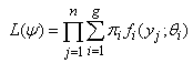 | (2) |
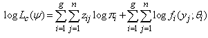
To estimate the parameter vector ψ we either maximize the likelihood in (2) or maximize the loglikelihood given in (3) below directly.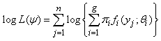 | (3) |
The likelihood in (2) can also be maximized using the EM (expectation maximization) algorithm. This is done by first introducing an observable or missing data vector z = (z1T, z2T,…, znT). The vector of indicator variables zj = (z1j, z2j,…, zgj)T is defined by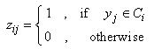 Instead of maximizing the likelihood in (2) above, the EM – algorithm can be used to maximize the likelihood in (4) or the loglikelihood in (5) which is often referred to as the complete-data loglikelihood.
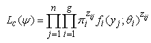 | (4) |
 | (5) |
2.2. Longitudinal Mixture Model
2.2.1. Likelihood Formulation and Parameter Estimation
Nagin (1999) uses a polynomial relationship model to relate age to the response. Let yjt be a binary response for subject j at time t. It is assumed that conditional on membership in group i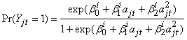 | (6) |
where  is the probability of the outcome of interest and
  is the age of subject j at time t. The coefficients
  and
and  determine the shape of the trajectory and are superscripted by i to indicate that the coefficients are allowed to vary across the different groups.Let yj = (yj1, yj2, …,yjm) denote the longitudinal sequence of observations for subject j. Conditional on being in group i, a subject’s longitudinal observations are assumed independent , thus
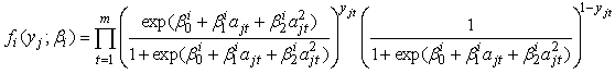 | (7) |
where  is the age of subject j at time t and
  is the response of subject j at time t (which is either zero or one). As described by Nagin (1999), the form of the likelihood for each subject j is given by
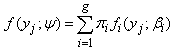 | (8) |
where  is the unconditional probability of observing subject j’s longitudinal measurements,
  is the probability of yj given membership in group i. The likelihood for the entire sample of n subjects is given by
 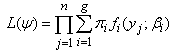 | (9) |
where g is the number of groups and πi is the probability of membership in group i. Each  is a set of parameters describing the ith group and ψ = (θ1, θ2, …, θg, π1, π2, …, πg) is the set of all parameters. Being probabilities (π1, π2, …, πg) must satisfy the constraints
  The likelihood in (9) can be maximized directly using PROC TRAJ. Maximization of this likelihood using the EM – algorithm requires introducing the missing data indicator z and obtaining the complete-data likelihood in (10).
  | (10) |
Substituting (7) into (10) and finding the log of the result gives the complete-data loglikelihood in (11). | (11) |
The E-step (expectation step) on the (k+1)th involves evaluating  where
where 
 This expectation only requires the evaluation of
 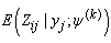 which is given by
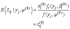 | (12) |
On the (k+1)th iteration, the M-step constitutes finding a value of ψ, that maximizes the expected loglikelihood, thus | (13) |
This is given by 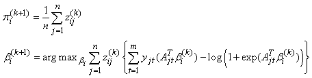 | (14) |
where  so that
  for
for  Since there is no closed form solution for
  , the maximization requires iteration. Starting from some initial parameter value
  , the E- and M-steps are repeated until convergence.
2.2.2. Estimation of Standard Errors
Standard errors of the parameter estimates are obtained from the inverse of the observed matrix. Unlike Newton-type methods, the EM-algorithm does not automatically provide an estimate of the covariance matrix of the maximum likelihood estimates. Louis (1982) derived a procedure for extracting the observed information matrix from the complete data loglikelihood when the EM-algorithm is used to find maximum likelihood estimates. McLachlan and Krishnan (1997) demonstrated the use of this procedure on a number of examples including its use on a mixture of standard normal distributions.According to the procedure, the observed information matrix  is computed as
  | (15) |
where 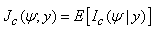 | (16) |
is the conditional expectation of the complete-data information matrix  given y and
 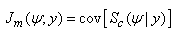 | (17) |
where  is the score vector based on the complete-data loglikelihood. The complete-data loglikelihood for a g-component mixture in (11) can be written in the form
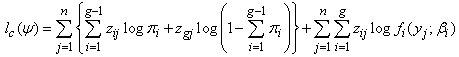 | (18) |
From (18) the complete-data information  is obtained as a 4g – 1 by 4g – 1 block-diagonal matrix given by
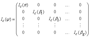 | (19) |
where  is a g – 1 by g – 1 matrix with diagonal elements
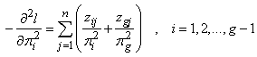 | (20) |
and off-diagonal elements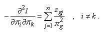 | (21) |
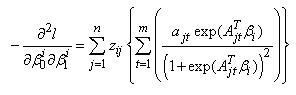
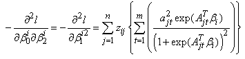
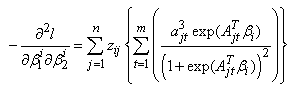
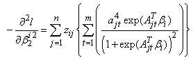
Each  is a 3 by 3 matrix given by
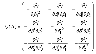 | (22) |
where 
 The score vector
  based on the complete-data loglikelihood is given by
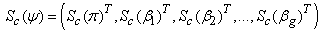 | (23) |
where 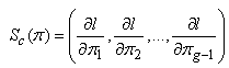 | (24) |
and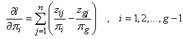 | (25) |
The score vector for each group  is given by
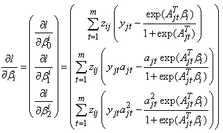 | (26) |
The conditional covariance of the score vector  is given by
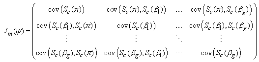 | (27) |
where  a g – 1 by g – 1 matrix,
 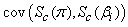 is a g – 1 by 3 matrix and
  is a 3 by 3 matrix for
  . Since we are taking the conditional covariance of the score vector given the vector y, we only need to evaluate E(Zij), Var(Zij) and Cov(Zij,Zkj) for
  , where Zij is a random variable corresponding to zij. Let
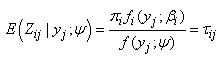 | (28) |
then 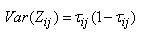 | (29) |
and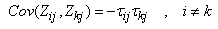 | (30) |
Using the expressions (28) to (30), the diagonal elements of the matrix  can be expressed as
 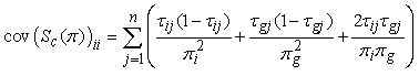 | (31) |
while the off diagonal elements can be expressed as 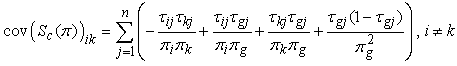 | (32) |
Similarly, the kth row of the matrix  is given by
 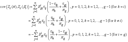 | (33) |
where 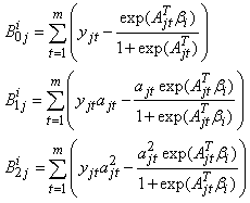 | (34) |
The covariance matrices  and
and  (for
(for  and
and  ) are respectively given by
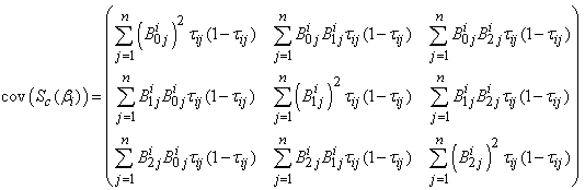 | (35) |
and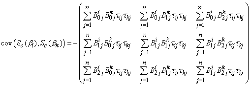 | (36) |
After running the EM algorithm until convergence, the parameter estimate  and estimated posterior probabilities
  are obtained. The variance estimate for
  is obtained from the inverse of the matrix
  with
with  in
in  and
and  in
in  replaced by
  .
.
3. Simulation Results
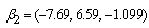
We consider simulation results for mixtures of two and three groups of longitudinal trajectories. Consider three groups of longitudinal trajectories with group parameters  and
and 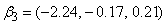 . These parameter values are calculated based on the trajectory shapes given in Figure 1 below. We consider a situation involving five time points where measurements are taken at times 1 to 5 (i.e.
 ). Using the above parameter estimates, a sequence of binary responses are generated for time points 1 to 5. Since the responses are assumed to be independent at each time point, the binary responses are generated independently at each time point. The binary response for the jth subject from group i at time t is generated with success probability
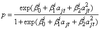 | (37) |
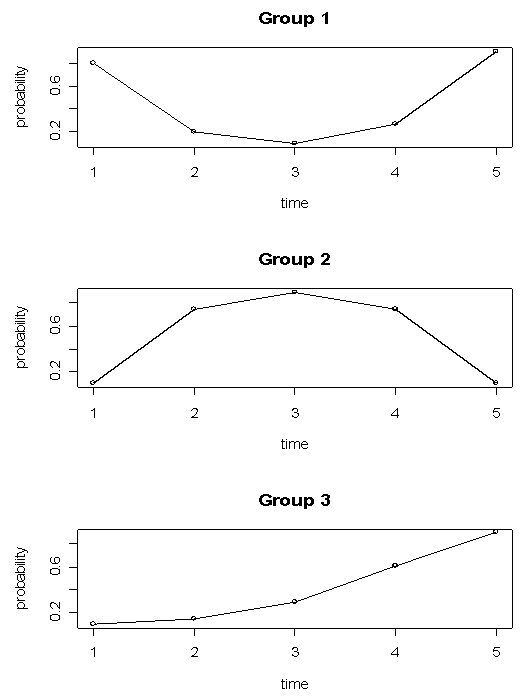 | Figure 1. Longitudinal trajectories for three groups |
For example, observations from group one at time point three are generated with success probability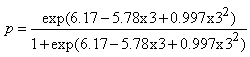 | (38) |
In the theoretical longitudinal trajectory groups given in Figure 1 below, time is plotted against the probability of having the characteristic of interest. If smoking was the characteristic of interest, for example, group one would represent a group of smokers who temporarily stop smoking for some time and then continue smoking again while group three would represent a group of subjects who are initially non-smokers who start smoking and continue smoking throughout the course of the study. In the simulation results that follow, results obtained using the EM algorithm explained in section 2 and PROC TRAJ are presented. For all the results obtained from the EM algorithm we present, the convergence criterion is based on changes in the maximized loglikelihood values. We stop the steps for the EM algorithm when the difference in the loglikelihoods is less than 10-8 for the model involving a mixture of two trajectory groups and 10-3 for the model involving a mixture of three trajectory groups.
3.1. Mixture of Two Trajectory Groups
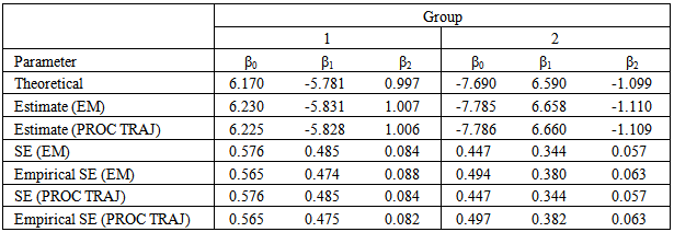
Consider 100 simulations of data sets of 500 observations from a mixture of two trajectory groups with group parameters 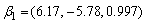 and
and  . For each simulation a total of 500 observations are generated – observations are generated from group one with success probability 0.32. The results are given in Table 1 and Table 2 below. Table 1 shows group parameter estimates, standard error estimates and empirical standard error estimates obtained from the EM algorithm and the PROC TRAJ procedure. The empirical standard errors reported in the table are sample standard deviations of the actual parameter estimates. Table 2 shows the estimates for the mixing proportions.
Table 1. Group parameter estimates and standard errors based on 100 simulations
 |
| |
|
Table 2. Average proportion parameter estimates based on 100 simulations
 |
| |
|
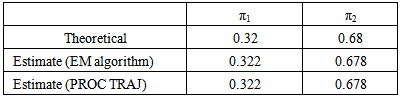
As can be seen from the tables, the estimated group parameter estimates and mixing proportion parameter estimates are very close to the theoretical values. It can also be seen that the standard errors obtained are comparable to the empirical standard errors.Table 3 shows the average number of EM steps and PROC TRAJ iterations required to obtain the maximized loglikelihood value correct to between 0 and 5 decimal places. From the table we see that the EM algorithm takes an average of about 8 steps to get to the integer part of the maximized loglikelihood value. In fact if we were only interested in obtaining the maximized loglikelihood value correct to two decimal places, the table shows that on average the EM algorithm requires only two additional steps after getting the integer part of the maximized loglikelihood value. On the other hand, the table shows that on average the EM algorithm requires 30 more steps to get from within zero to five decimal places of the maximized loglikelihood value. The table further shows that PROC TRAJ requires 23 iterations on average to get to the integer part of the maximized loglikelihood value and only an additional five iterations on average to get from within zero to five decimal places of the maximized loglikelihood value. Thus PROC TRAJ has a faster convergence rate once the procedure is within one or two decimal places of the maximized loglikelihood value.Table 3. Average number of steps/iterations required to get the loglikelihood correct to 0 to 5 decimal places for the EM Algorithm compared to PROC TRAJ based on 100 simulations
 |
| |
|
3.2. Mixture of Three Trajectory Groups
Unlike a mixture of two trajectory groups, a model with three groups is a little more complex as the results obtained tend to depend on the starting values used. This is especially more pronounced when the PROC TRAJ procedure is used. The EM algorithm tends to be a little less sensitive to starting values. As such starting values for three or more trajectory groups have to be carefully chosen.A procedure of coming up with starting values based on the logistic regression model is proposed. We propose dividing the data into groups based on the criterion described below and fitting a logistic regression model in each group and using the parameter values as starting values. For example, in a three group model, the data are initially divided into three groups and a logistic regression model is used to estimate the parameters in each of the three groups.The initial division of the data is based on the response at each of the five time points. One possible way of dividing the data is by looking at the response at two distinct time points. Since we are dealing with binary responses, there are four different possible patterns that naturally arise. The patterns are given in Table 4 below:| Table 4. Possible patterns for binary data at two distinct time points |
| | Pattern | Time1 | Time 2 | | 1 | 0 | 0 | | 2 | 0 | 1 | | 3 | 1 | 0 | | 4 | 1 | 1 |
|
|
If we were interested in fitting a model with four groups, we would make the initial division of the data based on the four patterns in the above table. For a three group model, one possible way of doing the division is by dividing the data into four groups and then merging the two smallest groups. One possible way of carrying out the initial division can be based on the first and last response values. To fit a model with more than four groups, we can look at three or more time points and then divide the data appropriately. After the data have been divided into groups, the proportions of the number of observations in each group can be used as the starting values for the proportions. For each group i, we fit a logistic regression model 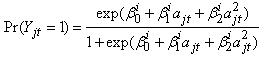 | (38) |
where  are the times at which observations are made on subject j. The parameter estimates
  and
and  are then used as starting values for group i.A total of 150 data sets of 800 observations from the three groups with parameters
 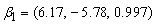 ,
,  and
and 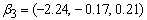 with mixing proportions
 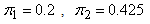 and
and  respectively, were considered. A closer look at the simulation results showed that the EM algorithm attains convergence to the first few decimal places of the maximised loglikelihood values quickly and then takes many steps to get the loglikelihood value correct to third and fourth decimal places. For all practical purposes we do not need to have a maximised loglikelihood value correct to five decimal places. As such the convergence criteria for the EM algorithm used for the three group model was 10-3. This means iterations in the procedure continues until the increase in the loglikelihood is less than 10-3. The simulation results are given in the following Table 5 and Table 6.
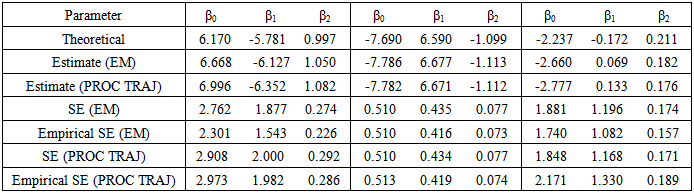
Table 5. Group parameter estimates and standard errors based on 150 simulations
 |
| |
|
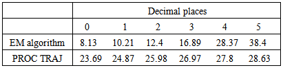
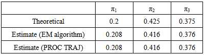
Table 6. Proportion parameter estimates obtained using the EM algorithm and PROC TRAJ compared to true parameter values
 |
| |
|
The results given in Table 5 and Table 6 show that the group parameter estimates and mixing proportion estimates obtained are close to the theoretical values though not as close as those obtained for the two parameter model given in Table 1 and Table 2. This may be as a result of the complexity of the model involved; the three group model is more complex than a two group model. The estimated standard errors obtained are comparable to the empirical standard errors.
4. Conclusions
In this article we have proposed the use of the EM algorithm to estimate parameters for a model involving a mixture of longitudinal trajectories. While the original mixture model of longitudinal trajectories (Nagin, 1999) can be applied to count, binary and psychometric data, this article only considered binary longitudinal data. Parameter estimation in this model involves estimating the mixing proportions, group parameter estimates and the corresponding standard errors. This is currently done using the Quasi-Newton method through a SAS procedure called PROC TRAJ as proposed by Jones et al. (2001). This paper therefore proposes an alternative way of carrying out the parameter estimation.The paper describes how to estimate the various parameters in the longitudinal trajectory mixture model using the EM algorithm. This is done by deriving expressions for the expectation steps (E-steps) and maximization steps (M-steps) for each of the parameters. Expressions for computing the variances for the parameter estimates are also derived. Simulation results comparing parameter estimates and standard errors obtained using the EM algorithm and the Quasi-Newton methods are presented.The simulation results show that results obtained by the two methods are basically the same especially for the two group model. Parameter estimation, however, tends to become difficult as the model becomes complex such as increasing the number of groups from two to three. There were no problems in parameter estimation for a two group model, however, there were some challenges fitting a three group model especially using the Quasi-Newton method. Simulation results suggest that the results obtained using the Quasi-Newton method are highly dependent on starting values and hence the proposal of logistic starting values. The EM algorithm appears to be less sensitive to starting values.Simulation results also suggest that the convergence rate of the EM algorithm is initially faster than that of the Quasi-Newton method as it requires a few EM-steps to get to the integer part of the maximized loglikelihood value and then requires a substantial number of EM steps to get the maximized loglikelihood value correct to a number of decimal places. As earlier stated under simulation results for the three group model, it may not matter a lot to get the maximized loglikelihood value correct to five decimal places, for example, as the parameter estimates do not reflect substantial changes. The simulation results also suggest that the Quasi-Newton method requires very few iterations to obtain the value of the maximized loglikelihood once the integer part of the maximized loglikelihood value is obtained.The proposed parameter estimation approach is therefore useful in the sense it is an alternative to the current method of parameter estimation. It can also be used with the current method to increase chances of getting the correct maximized loglikelihood value correct to a number of decimal places without a lot of iterations. The proposed approach may have problems with slow convergence rate beyond a certain value of the maximized loglikelihood especially for more complex models, however, it is less sensitive to starting values. As observed from the simulation results the current approach has a fast convergence rate but very sensitive to starting values. To solve the problems with the two approaches, the two approaches can be used together. Parameter estimation can begin with the proposed method since it is less sensitive to starting values and then the parameter estimates obtained can be used as starting values for the current method.
ACKNOWLEDGEMENTS
I would like to thank Prof K.S. Brown for his invaluable contribution to the work.
References
| [1] | Biernacki, C., Celeux, G. and Govaert, G. (2003). “Choosing starting values for the EM algorithm for getting the highest likelihood in multivariate Gaussian mixture models.” Computational Statistics and Data Analysis, 41, 561 – 575. |
| [2] | Blischke, W. R. (1962), “Moment estimators for the parameters of a mixture of two binomial distributions.” Annals of Mathematical Statistics, 33, 444 – 454. |
| [3] | Blischke, W. R. (1964),”Estimating the parameters of mixtures of binomial distributions.” Journal of the American Statistical Association, 59, 510 – 528. |
| [4] | Bremmer, J. M. (1978). “Algorithm AS 123: Mixtures of Beta distributions.” Applied Statistics, 27, 104 – 109. |
| [5] | Day, N. E. (1969). “Estimating the components of a mixture of normal distributions.” Biometrika, 56, 468 – 474. |
| [6] | Fraley, C. and Raftery, A. E. (2002).“Model-Based Clustering, Discriminant Analysis, and Density Estimation.” Journal of the American Statistical Association, 97, 611–631. |
| [7] | Jones, B. L., Nagin, D. S. and Roeder, K. (2001). “A SAS procedure based mixture models for estimating developmental trajectories.” Sociological Methods and Research, 29, 374 – 393. |
| [8] | Kao, J. H. K. (1959). “A graphical estimation of mixed Weibull parameters in life-testing electron tubes.” Technometrics, 1, 389 – 407. |
| [9] | Louis, T. A. (1982). “Finding the Observed Information Matrix when using the EM Algorithm.” Journal of the Royal Statistical Society B, 44, 226 – 233. |
| [10] | Marriot, F. H. C. (1975). “Separating mixtures of normal distributions.” Biometrics, 31, 767 – 769. |
| [11] | McLachlan, G. J. and Basford, K. E. (1988). “Mixture Models: Inference and Applications to Clustering.” New York: Marcel Dekker. |
| [12] | Nagin, D. S. (1999). “Analyzing developmental trajectories: A semiparametric group-based approach.” Psychological Methods, 4, 139 – 157. |
| [13] | O’Hagan, A., Murphy, T. B. and Gormley, I. C. (2012). “Computational aspects of fitting mixture models via the expectation–maximization algorithm.” Computational Statistics and Data Analysis, 56, 3843 – 3864. |
| [14] | Pearson, K. (1894). “Contributions to the theory of mathematical evolution.” Philosophical Transactions of the Royal Society of London A, 185, 71 – 1196. |
| [15] | Rider, P. R. (1961). “The method of moments applied to a mixture of two exponential distributions.” Annals of Mathematical Statistics, 32, 143 – 147. |
| [16] | Rider, P. R. (1962). “Estimating the parameters of mixed Poisson, binomial, and Weibull distributions by the method of moments.” Bulletin of the International Statistical Institute, 39, 225 – 232. |
| [17] | Symons, M. J. (1981). “Clustering criteria and multivariate normal distributions.” Biometrics, 37, 35 – 43. |
| [18] | Wolfe, J. H. (1970). “Pattern clustering of multivariate mixture analysis.” Multivariate Behavioral Research, 5, 329 – 350. |
 Abstract
 Reference
 Full-Text PDF
 Full-text HTML