-
Paper Information
- Next Paper
- Paper Submission
-
Journal Information
- About This Journal
- Editorial Board
- Current Issue
- Archive
- Author Guidelines
- Contact Us
International Journal of Statistics and Applications
p-ISSN: 2168-5193 e-ISSN: 2168-5215
2014; 4(3): 135-143
doi:10.5923/j.statistics.20140403.01
Bayesian Shrinkage Estimator for the Scale Parameter of Exponential Distribution under Improper Prior Distribution
 Abstract
 Reference
 Full-Text PDF
 Full-text HTML
Abbas Najim Salman , Raeeda Ali Shareef
Department of Mathematics-Ibn-Al-Haitham College of Education - University of Baghdad
Correspondence to: Abbas Najim Salman , Department of Mathematics-Ibn-Al-Haitham College of Education - University of Baghdad.
| Email: |  |
Copyright © 2014 Scientific & Academic Publishing. All Rights Reserved.
This paper deals with preliminary test single stage Bayesian Shrinkage estimator for the scale parameter (θ) of an exponential distribution when a guess value (θ0) for (θ) available from the past studies under the improper prior distribution and the quadratic loss function. The proposed estimators are shown to be a more efficient than the usual estimators θ when θ is close to θ0 in the sense of mean squared error (MSE). In which the expression for bias and mean squared error of the proposed estimator are derived. Numerical results for the bias and MSE are using different constants were involved in it which had been given as well as comparisons.
Keywords: Exponential Distribution, Maximum Likelihood Estimator, Improper Prior Distribution, Bayesian Estimator, Single Stage Shrinkage Estimator, Mean Squared Error, Relative Efficiency
Cite this paper: Abbas Najim Salman , Raeeda Ali Shareef , Bayesian Shrinkage Estimator for the Scale Parameter of Exponential Distribution under Improper Prior Distribution, International Journal of Statistics and Applications, Vol. 4 No. 3, 2014, pp. 135-143. doi: 10.5923/j.statistics.20140403.01.
Article Outline
1. Introduction
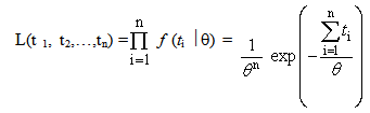
- One of the most useful and widely exploited model is the exponential distribution, Epstein [7] remarks that is the exponential distribution which plays as important role in life experiments as the part played by the normal distribution in agricultural experiments. It is applied in a very wide variety of statistical procedures. Among the most prominent applications were found in the field of life testing and reliability theories. The scale parameter (θ) is known as mean life time. The maximum likelihood estimator for θ is a sample mean which is unbiased and a minimum variance unbiased linear estimate.The one parameter exponential distribution has the following probability density function (p.d.f)
 | (1) |
 , where k (constant) had been known as a shrinkage weight function, 0 < k < 1, which is specified by the experimenter in advance according to his belief in θ0. He compared the estimator T with
  , in the terms of MSE. Another class of shrinkage estimators were bounded MSE and had a better performance than the usual estimator, which have been discussed in [9] and [10]. Bhattacharya and Srivastava [6] were used the antecedent prior estimate θ0 to propose an preliminary test single stage shrinkage estimator for θ as below
 | (2a) |
 =0 and
  =1.Also, several authors had been studied the general preliminary single stage Shrinkage estimator form (2a) is by taken many different choices for the shrinkage weight factors
  (i =1,2),
  . For example, it may be taken as
 | (2b) |
 ,
,  it may be constant or a function of
  in which to represents one's degree of belief in the prior estimate θ0, R is a suitable region in the parameter space which may be pretest region. See [1], [2], [3], [4], [8] and [12].The idea of this paper is concern with the development of preliminary single stage shrinkage estimators (2a) is for estimate the scale parameter of exponential distribution been using the Bayesian estimation technique under the improper of prior distribution and quadratic loss function. Various choices of shrinkage weight function had been considered as well as being pretest region R for complete samples. The expressions for Bias, Mean Squared Error and Relative Efficiency were derived. Numerical results for Bias and Relative Efficiency (R.Eff.) been given for a different constant involves in the estimators.
3. Bayesian Estimator
- Consider the one parameter exponential distribution (1), and assume the following improper prior distribution of θ;
 | (3) |
 | (4) |
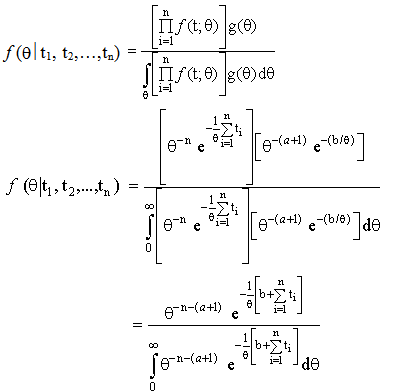 | (5) |
 | (6) |
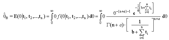 | (7) |
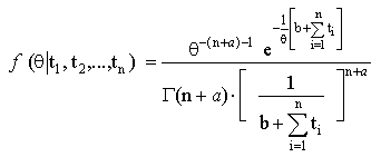
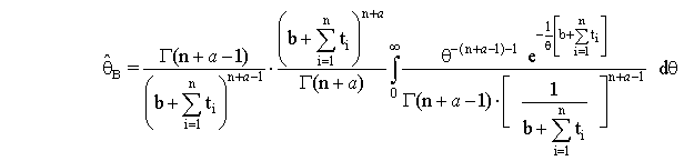 And by simple calculations, we get
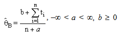 | (8) |
4. Preliminary Single Stage Bayesian Shrinkage Estimator 
- This section is concern with the pooling approach between shrinkage estimation which had been used a prior information about an unknown parameter as initial values and Bayesian estimation were uses a prior information about unknown parameter being a prior distribution for the scale parameter (θ) of exponential distribution were using specific shrinkage weight factors as well as pretest region (R) when a prior information about (θ) is available as initial value (θ0).General preliminary test single stage Bayesian Shrinkage (PSSBS) estimator were defined below
 | (9) |
 had been represented to Bayes estimator for θ is defined with equation (8), R which is suitable region (say pretest) and
 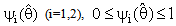 is shrinkage weight function which might be a function of
  (MLE) or a constant, See [2].
4.1. Preliminary Test Single Stage Bayesian Shrinkage Estimator 
- Using the form (9), the proposed PSSBSE
 had the following forms:
 | (10) |
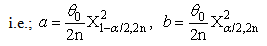
 (constant), 0 < k < 1;and suppose that a=0 and b= -1 in equation(8).where R is pre-test region of acceptance to size α for testing the hypothesis H0: θ = θ0 against the hypothesis HA : θ ≠ θ0 using the test statistic T
 in that
 | (11) |
 | (12) |
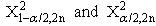 had been respectively a lower and an upper 100(α/2) percentile point of chi-square distribution with degree of freedom (2n).Also,
  refer to Bayes estimator,
  is MLE of θ and θ0 was a prior information of θ.The expressions for Bias [B(•)] and mean square error [MSE] of
  were represented respectively as follows:
 where
where  is the complement region of R in real space and f (
 ) is a p.d.f. of
  which has the following form
 | (13) |
 | (14) |
 | (15) |
 | (16) |
 | (17) |
 with respect to the classical estimator (
 ) is defined as below
 | (18) |
4.2. Preliminary Test Single Stage Bayesian Shrinkage Estimator 
- By using the form (9), which the proposed PSSBS estimator
 had the following forms:
 | (19) |
 (constant), 0 < k < 1;and suppose that a=0 and b= 0.The expressions for Bias [B(•)] and the Mean Squared Error [MSE] of
  were represented respectively as follow up:
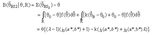 | (20) |
 | (21) |
5. Numerical Results
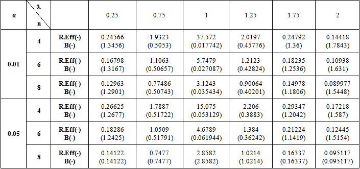
- The computations of relative Efficiency [R.Eff(•)] and the Bias ratio [B(•)] been used for the estimator
 (i=1,2).These computations were performed for α = 0.01,0.05,0.1, k = 0.01,0.1,0.3,0.5, λ = 0.1(0.1)1,2, n = 4,6,8,10,12. Some of these computations had been given in annexed tables. The observation mentioned in the tables lead to the following results:1. R.Eff(•) of
  are adversely proportional with the small value of α and those of n and k.2. R.Eff(•) of
  are maximum however when θ = θ0(λ = 1) for all α, n and k.3. R.EffB(•)is better than R.Effc(•) of
  .4. Bias ratio [B(•)] of
  are reasonably a small when is θ
  θ0, otherwise B(•) will be maximum for all α and n.5. B(•) of
  are a small compared with the small sample size (n) and also with the small α and k.6. Effective Interval [the values of λ that makes R.Eff. are greater than one] for
  is [0.5,1.5].7. The suggested estimator
  are more efficient than the estimators introduced by [6], [9] and [10] in the terms to Mean Squared Error (MSE).8. The suggested estimator
  is more efficient than the estimator
  in the sense of mean squared error (MSE).
|
 when k = 0.1
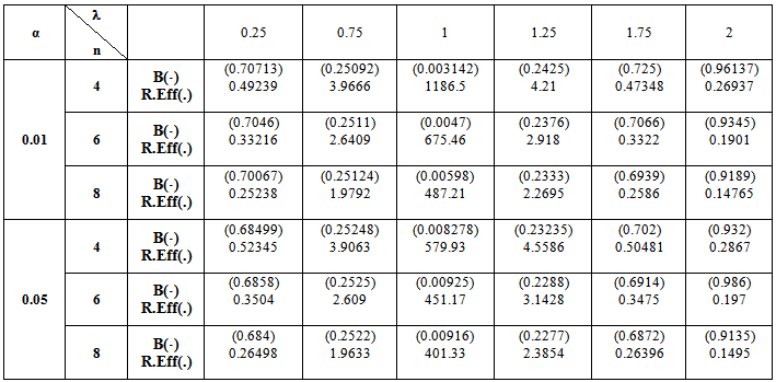
|
 when k = 0.3
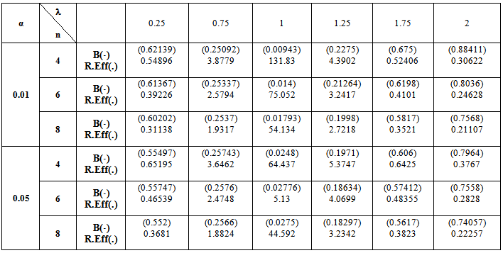
|
 when k = 0.5
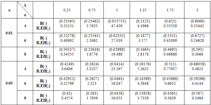
|
 when k = 0.1
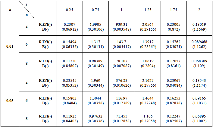
|
 when k = 0.3
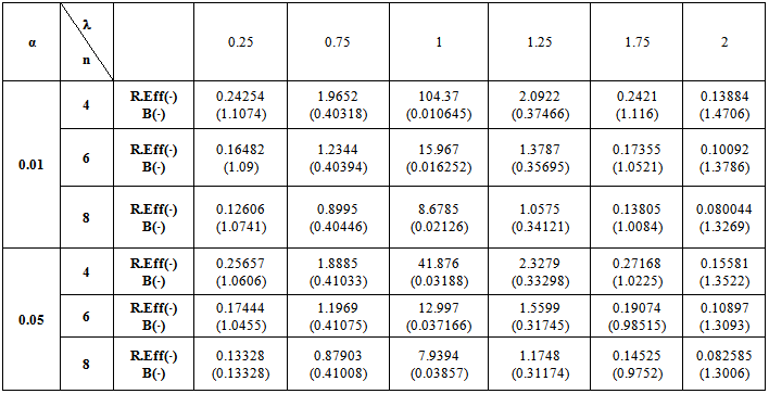
|
 when k = 0.5