Ijomah Maxwell Azubuike1, Opabisi Adeyinka Kosemoni2
1Dept. of Mathematics/Statistics, University of Port Harcourt, Rivers State
2Dept. of Mathematics/Statistics, Federal Polytechnic Nekede, Owerri Imo State
Correspondence to: Opabisi Adeyinka Kosemoni, Dept. of Mathematics/Statistics, Federal Polytechnic Nekede, Owerri Imo State.
| Email: |  |
Copyright © 2014 Scientific & Academic Publishing. All Rights Reserved.
Abstract
Cross product matrix approach is a more widely used least-squares technique in estimating parameters of a multiple linear regression. However, it is imperative to consider other forms of estimating these parameters. The use of singular value decomposition as an alternative to the widely known cross-product matrix approach as formed one of the basis of discussion in this paper. However, the use of cross product matrix have placed a lot of restrictions on the user of this technique which makes it difficult to estimate parameter values when the predictor variables seem to be highly correlated, this is often the case when Collinearity (Multi-collinearity) exists among the predictor variables. The consequence of this is that certain conditions that makes the cross product matrix applicable are not satisfied, hence the singular value decomposition approach enables users to resolve this difficult. With the aid of empirical data sets, both methods have been compared and difficulties encountered in the use of the former have been resolved using the latter.
Keywords:
Singular Value Decomposition, Cross product and Collinearity
Cite this paper: Ijomah Maxwell Azubuike, Opabisi Adeyinka Kosemoni, Singular Value Decomposition Compared to cross Product Matrix in an ill Conditioned Regression Model, International Journal of Statistics and Applications, Vol. 4 No. 2, 2014, pp. 124-133. doi: 10.5923/j.statistics.20140402.07.
1. Introduction
The use of cross product matrix for obtaining least squares estimates in multiple regression analysis has been in use for a long time. It is about the major statistical technique for “fitting equations to data”. However, recent works has also provided modifications of the techniques aimed at increasing its reliability as a data-analytic tool most especially when near-collinearity exists between explanatory variables. When perfect collinearity occurs, the model can be reformulated in an appropriate fashion. A different type of problem occurs when collinearity is near perfect Belsley et al (1980). Collinearity can increase estimates of parameter variance; yield models in which no variable is statistically significant even when the correlation coefficient is large; produce parameter estimates of the “incorrect sign” and of implausible magnitude; create situations in which small changes in the data produce wide swings in parameter estimates; and, in truly extreme cases, prevent the numerical solution of a model. These problems can be severe and sometimes crippling. Rolf (2002), stated that mathematically, exact collinearities can be eliminated by reducing the number of variables, and near-collinearities can be made to disappear by forming new, orthogonalized and rescaled variables. However, omitting a perfect confounder from the model can only increase the risk for misinterpretation of the influences on the response variable. Replacing an explanatory variable by its residual, in a regression on the others from a set of near-collinear variables, makes the new variable orthogonal to the others, but with comparatively very little variability. Owing to this lack of substantial variability, we are not likely to see much of its possible influence. Mathematical rescaling cannot change this reality, of course. To a large extent it is a matter of judgment what should be called a comparatively large or small variation in different variables and variable combinations, and this ambiguity remains when it comes to shrinkage methods for predictor construction, because these are not invariant under individual rescaling and other non-orthogonal transformations of variables. We could say that the ‘near’ in near-collinearity is not scale invariant.The purpose of this paper is to compare the singular value decomposition to that of cross product matrix approach in an ill conditioned regression in order to observe if both approaches vary according to the degree of collinearity among the explanatory variables. The rest of this paper is organized as follows: Section two discusses the methodology, Section three discusses the data analysis and results while concluding remarks are presented in Section four.
2. Methodology
The cross-product matrix least-squares estimates approach and singular value decomposition will be employed in obtaining the parameters of the model. A comparison of the two approaches will be looked into with a view of observing if the two approaches will enable us obtain the equal parameter estimates.The general linear model assumes the form  | (1) |
This model can also be written in the form  | (2) |
2.1. Cross-Product Matrix Approach for Obtaining Parameter Estimates
From equation (1) we form the equation below | (3) |
where  is a
is a  column vector of responses variable,
  is
is  matrix of
  predictor variables of
  observations,
  is a
is a  column vector and
  is a random error of
  dimension associated with
  vector. Y and X are known vectors (observations obtained from a data set), while
  and
and  are unknown vectors.As defined earlier the vectors;
 | (4) |
 | (5) |
 | (6) |
 | (7) |
From equation (2) the unknown vectors  and
and  will be obtained using the cross-product matrix; Therefore we rewrite (2) since E(e)=0 (Regression Analysis Assumption)
 | (8) |
Multiplying both sides of equation (8) by 
 | (9) |
From equation (9) we form | (10) |
Equation (10) forms matrices for obtaining the estimates of the parameters.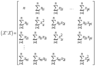 | (11) |
 | (12) |
From equation (10) it can be established that  is the variance/co-variance matrix of the parameters, which is a useful in testing hypotheses and constructing of confidence intervals.
2.2. Singular Value Decomposition Approach
Given  matrix X as earlier defined, it is possible to express each element
  in the following way:
 | (13) |
Hence by relation | (14) |
where  Equation (14) is known as the singular value decomposition (SVD) of matrix X. The number of terms in (15) is r which is the rank of matrix X; r cannot exceed n or p whichever is smaller.It is assumed that
  , and it follows that
  . The r vectors u are orthogonal to each other, as are the r vectors v. Furthermore, each of these vectors has unit length so that;
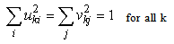 | (15) |
In matrix notation we have | (16) |
The matrix  is diagonal, and all
  are positive. The columns of the matrix U are the u vectors, and the rows of V’ are the v vectors of (12). The orthogonality of the u and v and their unit length implies the conditions
 | (17) |
 | (18) |
The  can be shown to be the square roots of the non zero eigenvalues of the square matrix
  as well as the square matrix
  . The columns of U are the eigenvectors of
  and the rows of V’ are the eigenvectors of
  . When
  it is known as a full-rank case. Each element of X is easily reconstructed by multiplying the corresponding elements of the
  matrices and summing the terms.From equation (3)
  We obtain
  | (19) |
Can be expressed also as Where
Where  is a
is a  matrix, that is a vector of r elements. Let us denote the vector by
  .
. | (20) |
 | (21) |
The matrix Y and the matrix U are known. The least squares solution for the unknown coefficients  is obtained by the usual matrix equation
 which, as a result of (17) becomes
 | (22) |
This equation is easily solved since  simply the inner product of the matrix Y with jth vector
  . It follows from (21) that
 But E
But E 
 | (23) |
Thus,  is unbiased. Furthermore, the variance of
  is
is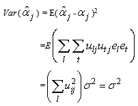 Hence
Hence | (24) |
Therefore the relationship between  and
and  is given by equation (20), which also holds for the least squares estimates of
  and
and 
 | (25) |
In (25),  has the dimension
  . Thus, given the
  values of
  , the matrix relation (25) represents r equations in p unknown parameter estimates
  . If r=p (the full-rank case). The solution is possible and unique.In this case V’ is a
  orthogonal matrix.Hence, the solution is given by
  | (26) |
It will be noted that  is
is  vector, obtained by dividing each
  by the corresponding
  .An important use of (26) aside from its supplying the estimates of
  as functions of
  , is the ready calculation of the variances of the
  . In general notation this equation is written as
  | (27) |
Also since the  are mutually orthogonal and have all variances
  we see that
 | (28) |
The numerators in each term are the squares of the elements in the first row of the V matrix and the denominators are the squares of  .
.
3. Data Analysis and Discussion
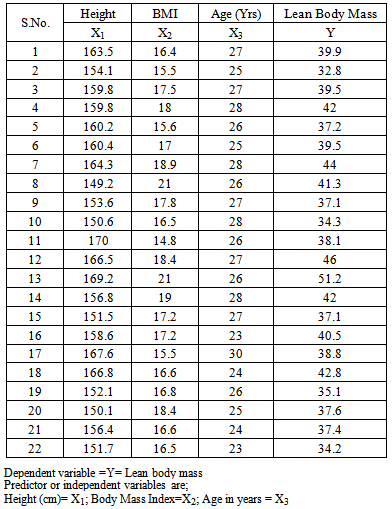
To simplify this exposition, we will consider the data below; which is on the details of measurements taken on 22 adults on lean body mass with height, body mass index and age given in the table below;Table 1
 |
| |
|
3.1. Application of Cross-Product Matrix Approach
From equations (7and 4) we define the matrices
 From equation (9) we obtain the cross-product of matrices
  and
and  , Using MATLAB
 We then obtain
 is the variance/co-variance matrix.
3.2. Singular Value Decomposition Approach
From equation (16)  Matrix X as defined earlier;Using MATLAB we obtain the Matrices
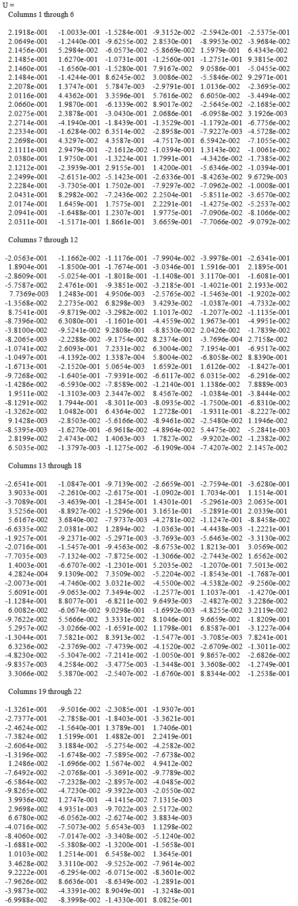
  For U (see appendix)
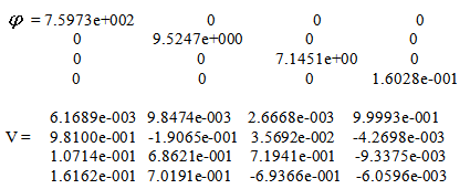 Therefore, if
  is the square roots of the non-zero eigen-values of the square matrix
  as well as the square matrix
  .The eigen-values of matrix
  using MATLAB is obtained below
 Redefining the Matrix
  by leaving the non-zero vectors; we have
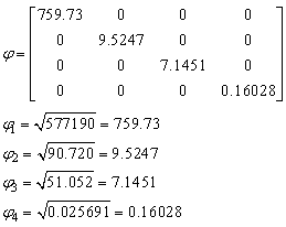 Similarly, the columns U are the eigen-vectors of
  and the rows of V’ are the eigen-vectors of
  .To obtain the parameter estimates, from equation (26)
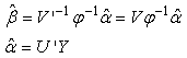 Where
Where  can be re-defined as column vectors U obtained from SVD (
 ) since r = 4, using MATLAB we have
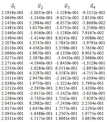
 Similarly,
  can be re-defined as row vectors V’ obtained from SVD (
 ) since r=4, using MATLAB we have
 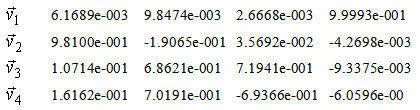 Recall


 Similarly, obtaining the variances we have;
 Using MATLAB
 For obtaining co-variances we have;
 In general we have;

3.3. Cross Product Matrix Approach Versus Singular Value Decomposition
We have been able to obtain regression model parameter estimates using both procedures and results are the same in both cases. However, one question most users of cross product matrix might ask is why go through the trouble of decomposing your predictor variables to several matrices when similar estimates are obtainable? The user of cross product matrix must bear in mind that estimates are only obtainable if and only if  matrix is nonsingular (i.e
 ). This is not often the case when predictor variables are linearly related, a situation often referred to as Perfect Collinearity or ill condition regression model.It then follows that, when
  is singular, we can use SVD to approximate its inverse by the following matrix;
 | (29) |
where Equation (29) is a modified form of equation (16).
4. Conclusions
From the analysis carried out using the cross product matrix and Singular value decomposition approach, parameter estimates are easy and uniquely determined using the cross product approach when there exist no near-collinearity between explanatory variables. On the other hand, singular value decomposition enables us to obtain similar estimates when no near-collinearity between explanatory variables though requires much more computational techniques than cross product matrix approach, but in addition, it enables us to handle the case of near-collinearity between the explanatory variables or ill conditioned regression models by applying the use of SVD to the matrix  thus making it possible for users of the cross product matrix approach to obtain parameter estimates after obtaining the inverse of SVD of the matrix
  .
.
APPENDIX
References
| [1] | Belsley D.A., Kuh E.; and Welsch,R.E. (1980), Identifying Influential Data and Sources of Collinearity, New York: John Wiley. |
| [2] | Rolf S., (2002), Collinearity, Encyclopedia of Environmetrics, John Wiley & Sons, Ltd, Chichester, 1, 365 – 366. |
 Abstract
 Reference
 Full-Text PDF
 Full-text HTML