Oyamakin S. O., Chukwu A. U.
Dept. of Statistics, University of Ibadan, Nigeria
Correspondence to: Oyamakin S. O., Dept. of Statistics, University of Ibadan, Nigeria.
| Email: |  |
Copyright © 2014 Scientific & Academic Publishing. All Rights Reserved.
Abstract
This paper proposed a hyperbolic exponential nonlinear growth model. Introducing a hyperbolic sine function into the Malthusian growth equation developed this. The solution, which is now a three-parameter model, was used in the modeling of height/diameter growth of PINE. Its ability in model prediction was compared the source model i.e. Malthusian growth model, an approach which mimicked the natural variability of heights/diameter increment with respect to age and therefore provides a more realistic height/diameter predictions using the coefficient of determination (R2), Mean Absolute Error (MAE) and Mean Square Error (MSE) results. The Kolmogorov Smirnov test and Shapiro-Wilk test was also used to test the behavior of the error term for possible violations. The mean function of top height/Dbh over age using the two models under study predicted closely the observed values of top height/Dbh in the hyperbolic exponential nonlinear growth models better than the ordinary exponential growth model.
Keywords:
Height, Dbh, Forest, Pinus Caribaea, Hyperbolic
Cite this paper: Oyamakin S. O., Chukwu A. U., On the Hyperbolic Exponential Growth Model in Height/Diameter Growth of PINES (Pinus caribaea), International Journal of Statistics and Applications, Vol. 4 No. 2, 2014, pp. 96-101. doi: 10.5923/j.statistics.20140402.03.
1. Introduction
In this paper, an alternative nonlinear growth model called the hyperbolic exponential growth model was introduced and compared with the existing classical exponential model built by Malthus. Growth is one of the well-known features in biological creatures (Burkhart and Strub, 1974). Growth models describe the changing size of something over time. Forest growth models are very useful for forest managers and forestry researchers in many respects. A forest growth model aims to describe the dynamics of the forest closely and precisely enough to meet the needs of the forester or forestry researcher.The process of developing a mathematical model is termed mathematical modeling. A model may help to explain a system and to study the effects of different components, and also to make predictions about behavior. A model may be deterministic or stochastic. A deterministic growth model gives an estimate of the expected growth of a system. Given the same initial conditions, a deterministic model will always predict the same result. A stochastic model attempts to illustrate natural variation by providing different predictions, each with a specific probability of occurrence. Deterministic and stochastic models serve complementary purposes. In forestry, deterministic models are effective for determining the expected yield, and may be used to indicate the optimum stand condition. Stochastic models may indicate the reliability of these predictions, and the risks associated with any particular regime. Both deterministic and stochastic predictions can be obtained from some models. Although stochastic models can provide some useful information not available from deterministic models, most of the information needed for forest planning and managements can be provided efficiently also with the use of deterministic models.Forest managers rely on growth and yield models to assess whether their short-term plans will meet long-term sustainability goals. Growth models assist forest researchers and managers in many ways. Some important uses include the ability to predict future yields and to help consider alternative cultivation practices. Models provide an efficient way to prepare resource forecasts, but a more important role may be their ability to explore management options and silvicultural alternatives EK, A.R., E.T. Birdsall, and R.J.Spear (1984). Growth models provide a reliable way to examine silvicultural and harvesting options, to determine the sustainable timber yield, and examine the impacts of forest management and harvesting on other values of the forest. Forest managers may require information on the present status of the resource (e.g. numbers of trees by species and sizes for selected strata), forecasts of the nature and timing of future harvests, and estimates of the maximum sustainable harvest. Forest simulation models or forest growth models are very useful for forest managers and forestry researchers in many respects. A forest growth model aims to describe the dynamics of the forest closely and precisely enough to meet the needs of the forester or forestry researcher. A mathematical description of a real world system is often referred to as a mathematical model. A system can be formally defined as a set of elements also called components. A set of trees in a forest stand, producers and consumers in an economic system are examples of components. The elements (components) have certain characteristics or attributes and these attributes have numerical or logical values. Among the elements, relationships exist and consequently the elements are interacting. The state of a system is determined by the numerical or logical values of the attributes of the system elements. Experimenting on the state of a system with a model over time is termed simulation (Kansal et al. 2000). Sustainable forest management relies to a large extent, measure on the predictions of the future conditions of individual stands which is achieved by predicting the increment from the current stand structure and updating the current values at each cycle of iteration using a functional growth model. Trees structural changes over time can be monitored and modeled under different cutting cycles, cutting intensities and optimal management policies can be arrived at based on the results of such simulation runs. 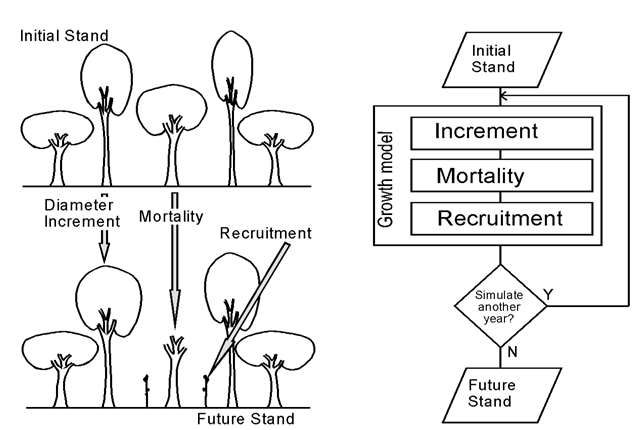 | Figure 1. Components of forest growth and the analogous representation in a stand growth model |
Growth models assist forest researchers and managers in many ways. Some important uses include the ability to predict future yields and to explore silvicultural options. Models provide an efficient way to prepare resource forecasts, but a more important role may be their ability to explore management options and silvicultural alternatives. For example, foresters may wish to know the long-term effect on both the forest and on future harvests, of a particular silvicultural decision, such as changing the cutting limits for harvesting. With a growth model, they can examine the likely outcomes (Myers 1996); both with the intended and alternative cutting limits, and can make their decision objectively. The process of developing a growth model may also offer interesting new insights into stand dynamics. The total height (Ht) of a tree is important for computing and estimating tree volume, stand characteristics and features through site index, but accurate measurement of this variable is time consuming. As a result, foresters often choose to measure only a few trees’ heights and estimate the remaining heights with height-diameter equations. Foresters can also use height-diameter equations to indirectly estimate height growth by applying the equations to a sequence of diameters that were either measured directly in a continuous inventory or predicted indirectly by a diameter-growth equation (Zeide 1993). The diameter-growth prediction method is very useful in modeling growth and yield of trees due to lack of approximations in measuring the diameter of trees. Curtis (1967) investigated several equations for Douglas-fir that included tree diameter outside bark at breast height (DBH) as an explanatory variable.
2. Materials and Methods
Consider a nonlinear model 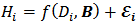 | (1) |
 Where
Where  is the response variable,
  is the independent variable, B is the vector of the parameters
  to be estimated
 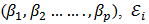 is a random error term,
  is the number of unknown parameters, n is the number of observation. The estimator of
 ’s are found by minimizing the sum of squares residual
  function.
  | (2) |
Under the assumption that the  are normal and independent with mean zero and common variable
  . Since
  and
and  are fixed observations, the sum of squares residual is a function of B, these normal equations take the form of
  | (3) |
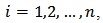
For . When the model is nonlinear in the parameters so are the normal equations consequently, for the nonlinear model consider the table 2, it is impossible to obtain the closed solution of the least squares estimate of the parameter by solving the
  normal equations describe in Eq (3). Hence an iterative method must be employed to minimize the
  (Draper and Smith 1981, Ratkowsky 1983, Marquardt 1963, Seber & Wild 1989, Fekedulegn 1996). The hyperbolic functions have similar names to the trigonometric functions, but they are defined in terms of the exponential function. The three main types of hyperbolic functions, and the sketch of their graphs are giving below.
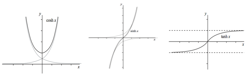 | Figure 2. Cosh Function, Sinh Function and Tanh Function |
Hence, the hyperbolic sine function and its inverse provide an alternative method for evaluating; If we make the substitution, then;
 Where the second equality follows from the identity cosh2(u) − sinh2(u) = 1 and the last equality from the fact that cosh(u) > 0 for all u. Hence;
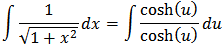
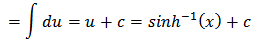 The following proposition is a consequence of the integral above i.e.
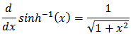 Also, using the substitution x = tan (u),
  , that
 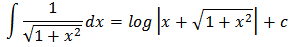 Since two anti-derivatives of a function can differ at most by a constant, there must exist a constant k such that
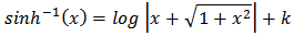 for all x. Evaluating both sides of this equality at x = 0, we have
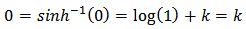 Thus k = 0 and
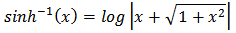 for all x. Since the hyperbolic sine function is defined in terms of the exponential function, we should not find it surprising that the inverse hyperbolic sine function may be expressed in terms of the natural logarithm function.
3. Hyperbolastic Exponential Growth Model (Hegm)
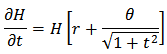 Separating the variables we have that;
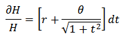 Integrating both sides we have that;
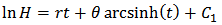 Hence,
 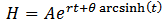 Therefore, we shall apply the two models below on Age-height and Age-Diameter of pines (pinus carean) growth;(1)
  , and
, and  (2)
(2)  , and
, and 
4. Results and Discussion
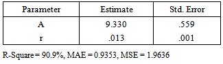
The tables 1-4 below show the estimated parameter for exponential and hyperbolic exponential growth model with their respective coefficient of determination (R2), MAE and MSE for age-height/age-diameter models. Also, tables 5 – 8 below show the ANOVA table of the two models compared and establish the significance of the models with the calculated F greater than the tabulated. Also, the mean square error computed from the ANOVA table shows that the proposed model is better compared to its source i.e Malthusian growth model. Table 1. Height Parameter Estimates using Exponential growth model
 |
| |
|
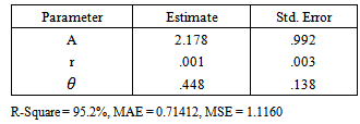
Table 2. Height Parameter Estimates using Hyperbolic Exponential growth model
 |
| |
|
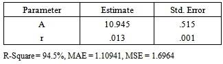
Table 3. Diameter Parameter Estimates using Exponential growth model
 |
| |
|
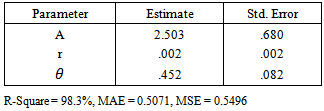
Table 4. Diameter Parameter Estimates using Hyperbolic Exponential growth model
 |
| |
|
Also, the predicted and observed height and diameter were plotted to show the relationship and how best the models predicted the observed data on height and diameter of pines. This is also shown in the figure below: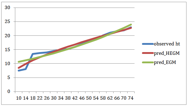 | Figure 3. Observed Height against Predicted HEGM & EGM |
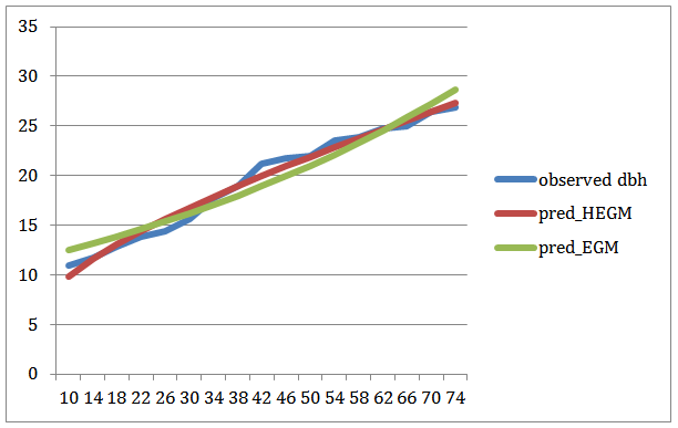 | Figure 4. Observed Diameter against Predicted HEGM & EGM |
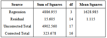
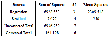
Table 5. ANOVA Table for the Hyperbolic Exponen-tial Growth model (Height)
 |
| |
|
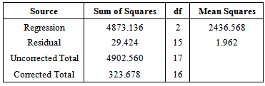
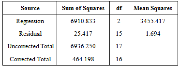
Table 6. ANOVA Table for the Exponential Growth model (Height)
 |
| |
|
Table 7. ANOVA Table for the Hyperbolic Exponen tial Growth model (Diameter)
 |
| |
|
Table 8. ANOVA Table for the Exponential Growth model (Diameter)
 |
| |
|
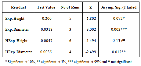
Testing for independence of errors (Run test) and Normality of Error (Shapiro-Wilk test)Two assumptions made in the models are:● Errors are independent● Errors are normally distributed.These assumptions were verified by examining the residuals. If the fitted models are correct, residuals should exhibit tendencies that tend to confirm or at least should not exhibit a denial of the assumptions.Hence, we tested the following hypotheses stated below;H0: Errors are independent (Using Runs Test)H1: Errors are not independentAndH0: Errors are normally distributed (Using Shapiro-Wilk test)H1: Errors are not normally distributedLet m be the number of pluses and n be the number of minuses in the series of residuals. The test is based on the number of runs(r), where a run is defined as a sequence of symbols of one kind separated by symbols of another kind. A good large sample approximation to the sampling distribution of the number of runs is the normal distribution with mean;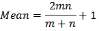 and,
and, 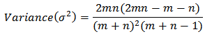 Therefore, for large samples like ours the required test statistic is;
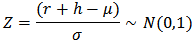 where,
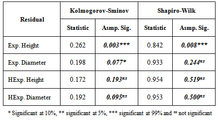
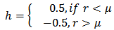 Also, the required test statistic for the test of normality (Shapiro-Wilk test) is given by;
 Where;
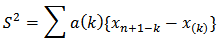 and,
and,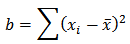 In the above, the parameter k takes the values;x(k) is the kth order statistic of the set of residuals and the values of coefficient a(k) for different values of n and k are given in the Shapiro-Wilk table. H0 is rejected at level α i.e. W is less than the tabulated value.
Table 9. Result of the test of independence of Residuals using Run Test
 |
| |
|
Table 10. Result of the test of normality of Residuals using K-S & S-W Tests
 |
| |
|
5. Conclusions
We have succeeded in introducing a new growth model using the hyperbolic function. The mean function of top height and Dbh over age using the Hyperbolic Exponential growth model predicted closely the observed values of top height and Diameter of Pines. However, large correlations of the estimated parameters do not necessary mean that the original model is inappropriate for the physical situation under study. For example, in a linear model, when a particular β (a coefficient) does not appear to be different from zero, it does not always imply that the corresponding x (independent variable) is ineffective; it may be that, in a particular set of data under study, x does not change enough for its effect to be discernible. In general, efficient parameter estimation can best be achieved through a good understanding of the meaning of the parameters, the mathematics of the model, including the partial derivatives, and the system being modelled. Hyperbolic Exponential model proposed can also be extended to lotka’s theorem about a stable population in Demography.
References
| [1] | Bertalanffy, L. von. 1957. Quantitative laws in metabolism and growth. Quantitative Rev. Biology 32: 218-231. |
| [2] | Brisbin IL: Growth curve analyses and their applications to the conservation and captive management of crocodilians. Proceedings of the Ninth Working Meeting of the Crocodile Specialist Group. SSCHUSN, Gland, Switzerland 1989. |
| [3] | Burkhart, H.E., and Strub, M.R. 1974. A model for simulation or planted loblolly pine stands. In growth models for tree and stand simulation. Edited by J. Fries. Royal College of Forestry, Stockholm, Sweden. Pp. 128-135. Model of forest growth. J. Ecol. 60: 849–873. |
| [4] | Curtis, R.O. (1967). Height-diameter and height-diameter- age equations for second-growth Douglas-fir. For. Sci. 13: 365-375. |
| [5] | Draper, N.R. and H. Smith, 1981. Applied Regression Analysis. John Wiley and Sons, New York. |
| [6] | Fekedulegn, D. 1996. Theoretical nonlinear mathematical models in forest growth and yield modeling. Thesis, Dept. of Crop Science, Horticulture and Forestry, University College Dublin, Ireland. 200p. |
| [7] | EK, A.R. ,E.T. Birdsall, and R.J.Spear (1984). As simple model for estimating total and merchantable tree heights. USDA. For. Serv. Res. Note NC-309.5p. |
| [8] | Kansal AR, Torquato S, Harsh GR, et al.: Simulated brain tumor growth dynamics using a three dimentional cellular automaton. J Theor Biol 2000, 203:367-82. |
| [9] | Khamis, A. and Z. Ismail, 2004. Comparative study on nonlinear growth curve to tobacco leaf growth data. J. Agro., 3: 147 – 153. |
| [10] | Kingland S: The refractory model: The logistic curve and history of population ecology. Quart Rev Biol 1982, 57: 29-51. |
| [11] | Marusic M, Bajzer Z, Vuk-Pavlovic S, et al.: Tumor growth in vivo and as multicellular spheroids compared by mathematical models. Bull Math Biol 1994, 56:617-31. |
| [12] | Marquardt, D.W., 1963. An algorithm for least squares estimation of nonlinear parameters. Journal of the society for Industrial and Applied Mathematics, 11: 431 – 441. |
| [13] | Myers, R.H. 1996. Classical and modern regression with applications. Duxubury Press, Boston. 359p. |
| [14] | Nelder, J.A. 1961. The fitting of a generalization of the logistic curve. Biometrics 17: 89-110. |
| [15] | Olea N, Villalobos M, Nunez MI, et al.: Evaluation of the growth rate of MCF-7 breast cancer multicellular spheroids using three mathematical models. Cell Prolif 1994, 27:213-23. |
| [16] | Philip, M.S., 1994. Measuring trees and forests. 2nd Edition CAB International, Wallingford, UK. |
| [17] | Ratkowskay, D.A., 1983. Nonlinear Regression modeling. Marcel Dekker, New York. 276p. |
| [18] | Seber, G. A. F. and C. J. Wild, 1989. Nonlinear Regression. John Wiley and Sons: NY. |
| [19] | Vanclay, J.K. 1994. Modeling forest growth and yield. CAB International, Wallingford, UK. 380p. |
| [20] | Zeide B (1993): Analysis of growth equations. Forest Sci 1993, 39:594-616. |
 Abstract
 Reference
 Full-Text PDF
 Full-text HTML