1. Introduction

Recently, forecasting of future observations based on time series data has received great attention in many fields of research. Several techniques have been developed to address this issue in order to predict the future behaviour of a particular phenomenon. The traditional approach based on Box and Jenkins' Autoregressive Integrated Moving Averages (ARIMA) models is commonly used because the resulting models are easy to understand and interpret. Support vector machines (SVM) and artificial neural networks (ANN) are alternative methods that can be used for forecasting in nonlinear time series and can overcome the problems of nonlinearity and nonstationarity. The use of SVM and ANN is increasing rapidly because of their ability to form complex nonlinear systems for forecasting based on sample data. In particular, in recent years, SVM and ANN have been applied in economic forecasting to predict stock market indicators in line with economic growth in various countries[1]. When fitting ARIMA models to economic and financial data that are either nonlinear or non-stationary time series, the results of forecasting are expected to be inaccurate. The forecast values tend to converge to the mean of the series after a few forecast values. Thus, alternative forecasting methods such as SVM need to be examined on non-linear and non-stationary time series.

The research problem in this study involves the applicability of the SVM method and its ability to forecast financial time series data; to investigate this, we compare SVM with those of the ARIMA and ANN techniques. The data used in this investigation is a time series that represents the daily scores of Al-Quds index of the Palestine Stock Exchange (PSE), published in the Palestine Stock Exchange [2]. The number of observations in the series is 1,321, representing daily scores in the period from August 1, 2007 to December 31, 2012, a period which includes the recent economic crises in the global financial market. The PSE operates five days per week, excluding national and religious holidays. Al-Quds index is the main indicator used to describe changes in stock prices in the market. This is an index number that measures the overall level of rise and decline in the prices of companies trading on the PSE. It is easy to see that the time series is not a stationary one.

Several studies have been conducted on the comparison between ARIMA models, SVM, and ANN in forecasting using time series data. Most of these studies have been data-based and many have used economic data. Kuan and White[3] discussed the possibility of using ANN for economic variables and the usability of traditional time series models, and emphasized the similarities between the two methods. In a similar study, Yao and Tan[4] used neural networks to predict several kinds of long-term exchange rates, whereas Tkacz[5] compared the forecasting abilities of time series models, linear models, and ANN models using Canadian gross domestic product (GDP) data and financial variables. Zhang[6] used a hybrid approach that combined the ARIMA and ANN models. Junoh[7] forecast the GDP of the Malaysian economy using information based on economic indicators. Mohammadi, et al.[8] compared several methods of forecasting the spring inflow to the Amir Kabir reservoir in the Karaj river watershed. Rutka[9] conducted a study to forecast network traffic using ARIMA and ANN. Some of these studies showed that ANN has limitations, such as an overtraining problem that emerges from the implementation of empirical risk minimization principles, making it fall into a local optimal solution. It is also necessary to select a large number of controlling parameters, which is very difficult to carry out.

SVMs were originally developed by Vapnik[10] for pattern recognition problems to provide a novel approach to improve the generalization property of neural networks. Recently, with the introduction of the e-insensitive loss function, SVMs have been extended to solve nonlinear regression, classification, and time series forecasting problems[11, 12, 13, 14]. SVMs’ ability to solve nonlinear regression estimation problems makes it a promising technique in time series forecasting[15, 16]. This has become a topic of intense interest due to its successful application in classification and regression tasks. Studies on SVM have shown some success in application to certain fields, such as pattern recognition and function regression. In terms of the application of SVM to financial time series forecasting, Kim[17] applied SVM to predict the stock price index for South Korea, while Tay & Cao[18] used SVM to predict five kinds of exchange rates, including GBP/USD, for the purpose of comparing between SVM and neural networks.

In this paper, we compares the performance of SVM with the ARIMA models and ANN learning theory, using a real-world dataset to train the models and to create a two-month forecast (10% of the number of observations). The results show that the tendencies of the predicted value curve using SVM are basically identical to those of the actual value curve. In addition, since there is no structured way to choose the optimal parameters of SVM, this study investigates the variability in performance with respect to the parameters.

2. Artificial Neural Networks

Rosenblatt[19, 20] developed the first single feed-forward network. Here, the output obtained from this single layer was the weighted sum of various inputs. A major development in ANN occurred when Cowan[21], introduced new functions, such as activation of the smooth sigmoid function, which have the capacity to deal with nonlinear functions more effectively than the learning process “perceptron” model. The procedure which uses the gradient-descent learning technique for multilayer feed-forward ANN is known as back-propagation, or the generalized delta rule, as set forth by Rumelhart, et al.[22] and developed by Zou et al.[23]. Initial weights are selected randomly between –1 and +1 and the power of NN models largely depends on how their layer-connection weights are adjusted over time. The weight adjustment process is known in NN methodology as training of the network. The objective of the training process is to update the weights in such a way as to facilitate learning of the patterns inherent in the data. The data is divided into two groups—the training group and the test group, where the training group is used to estimate the weights in the model.

The network outputs depend on the input units, hidden units, weights of the network, and the activation function. The ANN method uses the error or cost function to measure the difference between the target value and the output value. The back-propagation method takes the network error and propagates it backward into the network. Errors are used at each neuron to update the weights. The weights of the network are frequently adjusted in such a way that the error or objective function becomes as small as possible.

The output of ANN, assuming linear output neuron j, a single hidden layer with h sigmoid hidden nodes, and an input variable (x_i), is given by:

(1)

where g(.) is the linear transfer function of output neuron k and b_k is its bias; w_j is the connection weight between hidden layers and output units; and f(.) is the transfer function of the hidden layer.

Transfer functions can take several forms. The most widely used transfer functions are:

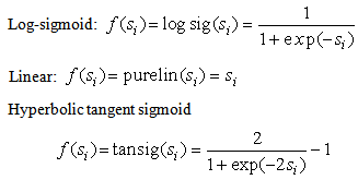(2)

where is the input signal, referred to as the weighted sum of incoming information.

The gradient descent method is utilized to calculate the weights of the network and to adjust the weight of interconnection to minimize the sum of the squared error (SSE) of the network. This is given by:

(3)

where and are the true and predicted output vectors, respectively, of the k^th output node. The constant ½ is used to facilitate computation of the derivative for the error function, which is essential in estimating the parameters[24].

For a univariate time series forecasting problem, the inputs of the network are the past lagged observations and the output is the predicted value [25]. Hence, ANN can be written as:

(4)

where w is a vector of all parameters and g(.) is a function determined by the network structure and connection weights. For more detailed information on the use and application of ANN for a time series, see Okasha & Yassin[26], and Tseng, Yu & Tzeng[27].

3. Support Vector Machines

SVM is used for a variety of purposes, particularly classification and regression problems. SVM can be especially useful in time series forecasting, from the stock market to chaotic systems[28]. The method by which SVM works in time series is similar to classification: Data is mapped to a higher-dimensional space and separated using a maximum-margin hyperplane. However, the new goal differs in that our goal is to find a function that can accurately predict future values[29].

Consider a given training set of n data points with input data , where p is the total number of data patterns and the output is . Generally, the idea of building SVM to approximate a function involves mapping the data x into a high-dimensional feature space via nonlinear mapping and performing a linear regression in the feature space. SVM approximates the function in the following form:

(5)

where, φ(x) represents a high-dimensional feature space that is nonlinearly mapped from the input space x[30]. The coefficients w and b are estimated by minimizing the following function:

(6)

subject to the following constraints:

(7)

This gives:

(8)

To estimate w and b, the above equation is transformed to the prime function below by introducing the positive slack variables ξ and ξ* as follows:

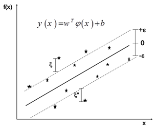Minimize

(9)

subject to the constraints:

The first term (1/2) in Eq. (9) is the weights vector norm, y_i is the desired value, and C is referred to as the regularized constant, determining the tradeoff between the empirical error and the regularized term. ε is called the tube size of SVM and is equivalent to the approximation accuracy placed on the training data points. Here, the slack variables ξ and ξ* are introduced. Using Lagrange multipliers and exploiting the optimality constraints, the decision function given by Eq. 9 takes the following explicit form:

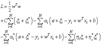(10)

with the constraints:

,

This can also be expressed in the form:

(11)

or more generally as:

(12)

where is defined as the kernel function[31, 32]. The value of the kernel is equal to the inner product of two vectors, X_i and X_j, in the feature space φ(x_i) and φ(x_j), that is, . Typical examples of the kernel function are:

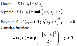
Here, γ, r, and d are kernel parameters; the kernel parameter need to be chosen carefully, as they implicitly define the structure of the high dimensional feature space φ(x) and thus controls the complexity of the final solution [33].

4. Application of the Box-Jenkins Methodology

The available time series data was composed of 1,321 observations representing Al-Quds daily stock price index for Palestine. The series was transformed using natural logarithms to stabilize the time series. Figure 1 represents the original time series and indicates that the time series was non-stationary and involved a sharp decline in stock market indices at the end of 2008; this was a period of worldwide economic crisis, which influenced all global financial markets. The natural logarithms of the series are displayed in Fig. 2 and the first order differences of the natural logarithms are shown in Fig. 3. No clear seasonal fluctuations in the series are observed, and the seasonal effects, if any, are disregarded.

Figure 1. Al-Quds Index Daily Data

Figure 2. The Logarithms of Al-Quds Index Daily Data

Figure 3. The 1st Differences of the Logarithms of Al-Quds Index

The sample autocorrelation and partial autocorrelation functions of the transformed Al-Quds index of the PSE time series, as shown in Fig. 4 and 5, indicated that the series had been stabilized, the transformed series was stationary, and some autocorrelations were significantly different from zero.

The stationarity of the transformed series was tested using Kwiatkowski, et al.[34] method, and the results indicated that the KPSS level was 0.1542, while the truncation lag parameter was 8, and the p-value was approximately 0.1. This indicates that the first difference of the natural logarithms of Al-Quds index of PSE series was stationary.

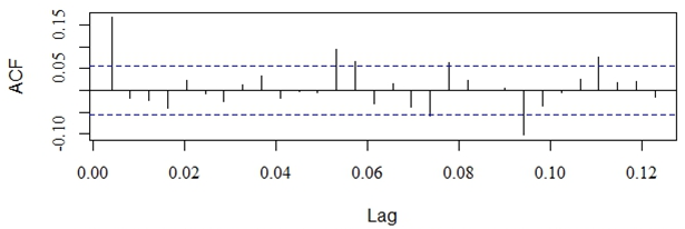Figure 4. The Autocorrelation Function of the Differenced Logarithms of the Series

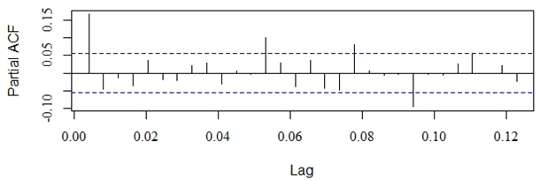Figure 5. The Partial Autocorrelation Function of the Differenced Logarithms of the Series

To fit the Box-Jenkins ARIMA model for the transformed series, we identified the orders p and q of the ARIMA model while fixing d at 1. The correlogram of the transformed series given in Fig. 4 and 5 above enables us to identify the values of these parameters. In this correlogram, we noted a significant autocorrelation and partial autocorrelation at lag 1. There are several graphical tools to facilitate identification of the ARMA orders. These include the corner method[35] and the extended autocorrelation (EACF) method[36, 37].

We applied the EACF method to the underlying differenced time series and compared the results of different estimates of p and q. The result of this comparison was that an appropriate model for the series could be ARIMA(0,1,1), ARIMA(1,1,2), or ARIMA(2,1,2). Therefore, the parameters for the three models were estimated, and the best model that could predict future values for stock prices among the models was identified. The results of this analysis revealed that the best model is ARIMA (0, 1, 1), since this had the lowest Akaike information criterion (AIC), and Bayesian information criterion (BIC).

The parameters of the ARIMA(0,1,1) model, as the best one, were estimated and the following model was obtained:

with AIC = -7717.59 and RMSE= 0.0282, where Y_t denotes the differenced natural logarithm of Al-Quds index of the PSE series. Note that the intercept was omitted from this model, since it was not significant and equalled zero.

Figure 6 displays three diagnostic tools for the fitted ARIMA(0,1,1) model. These are plots of the standardized residuals, the sample ACF of the residuals, and the p-values for the Ljung-Box test statistic for a whole range of values of K from 2 to 12. The horizontal dashed lines at 5% help determine the size of the p-values. These plots and the significance test of the coefficients suggest that the ARIMA(0,1,1) model fits the natural logarithms of Al-Quds index of the PSE time series adequately.

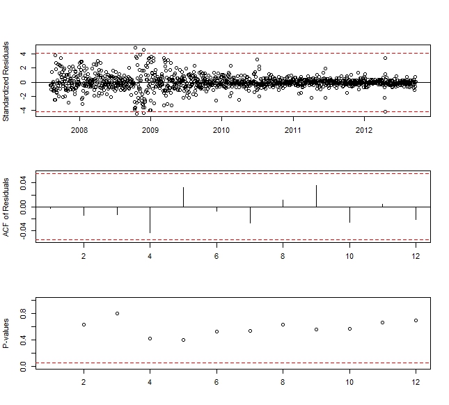Figure 6. Diagnostic Plots for the Residuals of the ARIMA(0,1,1) Model

Using the model in Eq. 13 above to forecast two-month future values yields, the forecast values displayed in Fig. 7 were obtained. The first two values were close to the actual values, while the rest quickly settled to the mean of the series; the 95% forecasting confidence limits contained all of the actual values. This shows that ARIMA models may be suitable for forecasting a few, but not many, future values.

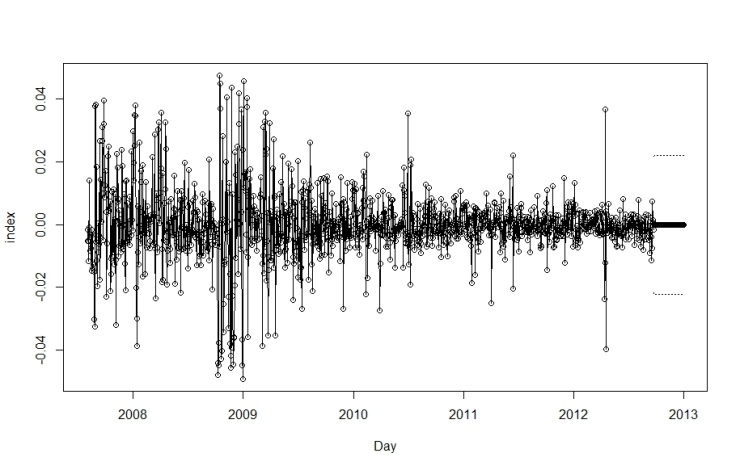Figure 7. Actual, Forecast and Forecast Limits for Differenced Logarithms of the Series

5. Fitting the Artificial Neural Network Model to the Data

This section focuses on fitting the ANN model described in Section 2 into the time series data for Al-Quds daily stock price index for Palestine. The data had 1,321 points, as shown in Fig. 1 and described in section 4. The number of observations in the training set was the same as the number of observations used in fitting the ARIMA model. That is, 90% (1,255 observations) of the series was considered a training set, and 10% (66 observations— representing more than a two-month period) was used as a test set. We assumed a continuous learning rate throughout the training of the network. R statistical software was used for all computations.

The selection of hidden layers for the network is not straightforward. When the number of hidden layer units is too small, correlation of the output and input cannot be assessed properly, and errors increase. However, when the number of hidden layer units is sufficiently large, unrelated noise and the correlation of both input and output can be examined, as the error increases accordingly. Many methods have been developed to identify the number of hidden layer units, but there is no ideal solution to this problem[38]. Therefore, in our analysis, we started with one hidden layer and gradually increased the number to 15 layers; we then attempted to find the network with the least RMSE for the residuals.

Since the series may also contain seasonality effects, different numbers of seasonal lags were used as inputs. When the feed-forward back-propagation network for the stock price index data was applied with one unit in the hidden layer associated with different values of lags and different learning rates, 90 results produce 90 networks. The best network with the minimum RMSE of the residuals in the various runs with different numbers of seasonal lags was that with one unit in the hidden layer and five seasonal lags. The minimum RMSE of the natural logarithms of Al-Quds index of the PSE for the final network equalled 0.02990. Taking into consideration the independence of the learning rates, the number of lags considered and the number of hidden layers, the RMSE value did not change a great deal.

Using the above ANN model, we obtained the forecasting results for Al-Quds index of the PSE time series as shown in Fig. 8. Moreover, through this figure we can observe that the values of forecasting were almost identical to the actual values of the time series, although ANN does not require the time series to be stationary.

Figure 9 shows the residuals of the final network and indicates that they were very small, with the majority close to zero, and most falling in the interval between -0.05 and 0.05. We may conclude that the best network to forecast the logarithms of the Al-Quds index of the PSE time series is that which uses the back-propagation algorithm with 15 units in the hidden layer, five seasonal lags used as inputs, and a learning rate of 0.01.

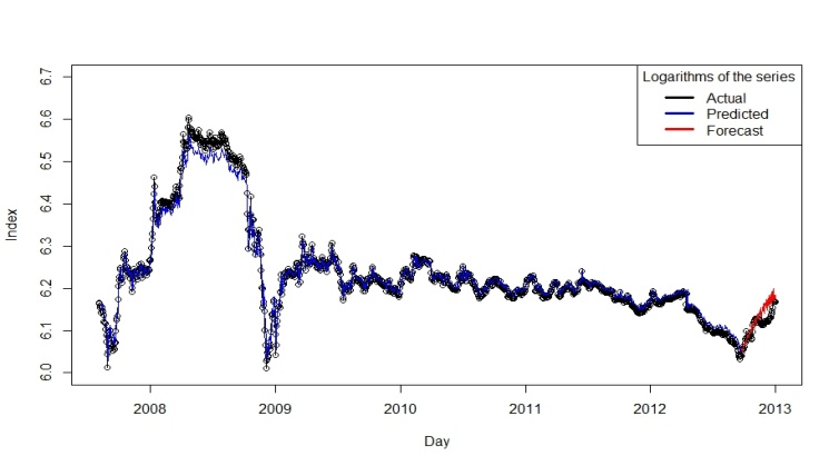Figure 8. Observed and Fitted Values of the Logarithms of the Series Using ANN

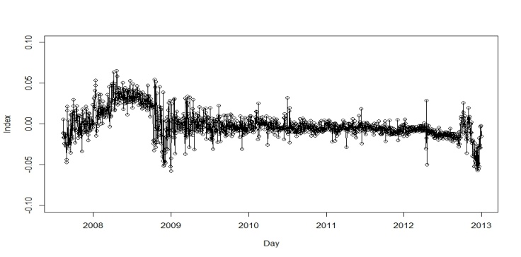Figure 9. Residuals of the ANN model of the Logarithms of the Series

6. Fitting the SVM to Data

The time series consisted of 1,321 points of daily Al-Quds indices of the PSE, as shown in Fig. 1. The series was transferred to natural logarithms to stabilize its variance, as shown in Fig. 2. First, 90% of the points in the series were used for training and the rest for testing the SVM. Ten-fold cross-validation was also performed.

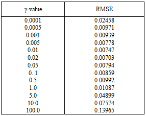
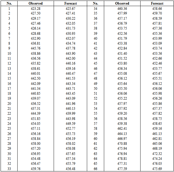
Now, given a time series , to make forecasting about it using SVM, the time series needed to be transferred into an autocorrelated dataset. That is to say, if is the goal value of forecasting, the previous values should be the correlated variables of the input. From this, we were able to map the autocorrelated input variables to the goal variable, . Here p is an embedding dimension. We considered the effect of the forecasting horizon and the embedding dimension on the performance of SVM. As to the choice of embedding dimension, this needed to be made in accordance with practical problems. Transferring the data in this way, we obtained the time series data suitable for SVM learning. The prediction performance was evaluated using RMSE.

Because we did not know the optimal embedding dimension p, we first had to determine this value. With the other conditions fixed, we used p={2,3,4,5,6,7,8,9} to carry out our preliminary experiments. From these experiments, we found that when p=5, RMSE was the lowest, so we concluded that five-days lagged daily indices was most suitable for forecasting the next-day’s index. We divide the time series data into two parts. The first included 1,256 points (90% of the series), which were used for both training and validation—to train the SVM and to find its optimal parameters. The test set was composed of the remaining 66 data points (10% of the series) which was used to check the predictive power of SVM.

Since there is no structured method for selecting the free parameters of SVMs, the generalization error and number of support vectors with respect to C and ε were examined. The kernel parameters γ and C were selected based on the validation set. RMSE and the number of support vectors with respect to the free parameters were investigated. In this investigation, the Gaussian function was used as the kernel function of the SVMs. Our experiments showed that a width value of the Gaussian function of γ=0.02 produced the best possible results. Figures 10 shows the logarithms of the series together with its predicted values for the training set and the forecast values of the test set, with the values of RMSE indicated below each figure for different experimental values of γ. C and ε were arbitrarily set at 10 and 1,000, respectively. Table (1) shows the values of the RMSEs at various experimental values of γ with C fixed at 100. The table shows that when γ ϵ (0.00001, 0.02), the RMSE decreases as γ increases, while γ ϵ (0.02, 10000), it increases as γ increases. This indicates that too small a value of γ ϵ (0.00001, 0.02), or too large a value of γ ϵ (0.02,10000) can cause the SVM to under-fit. An appropriate value for γ would be approximately 0.02 for this time series. This is because the value of γ=0.02 produce the minimum RMSE and hence prove to be the best possible value for γ and provide the best possible forecasts. Only the results of γ are illustrated; the same approach can be applied to the other two parameters.

Table 1. Values of the RMSE for various experimental values of γ with C fixed at 100

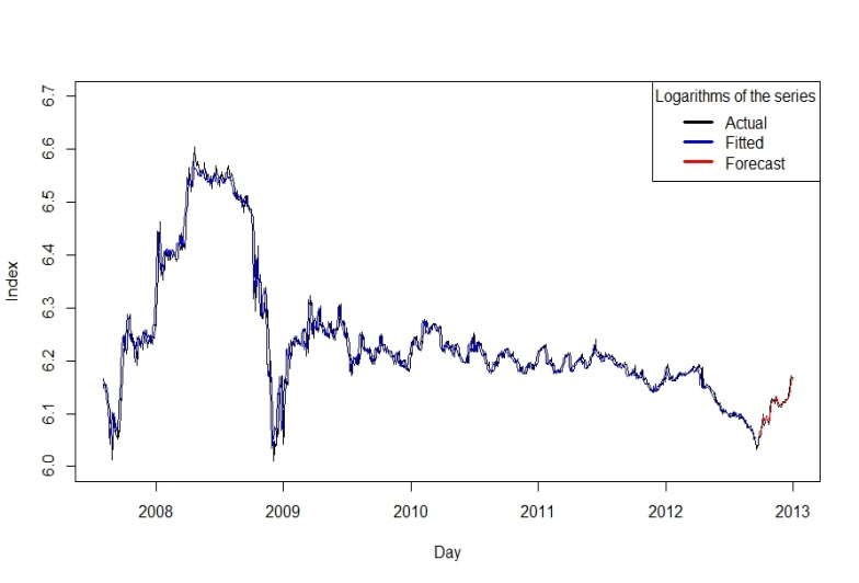Figure 10. Observed and Fitted Values of the Logarithms of the Series Using SVM (γ=0.02)

Table 2. Observed and Forecasted Values of Daily Scores of Al-Quds Index for 66 Days at End of 2012 Using the Final SVM

Summing up the analysis above and after several rounds of testing, we identified γ = 0.02, C = 100, and ε = 0.001 as the best selections for our experiment, and used these parameters to train the model again. Following this, we were able to predict the test set. The final result was RMSE = 0.00703, with a value of γ = 0.02. Figure 10 gives a comparison of forecast values with actual values, while Table 2 shows actual observed and forecast values of the daily scores of Al-Quds index of the PSE for 66 points at the end 2012, using consequent one-step-ahead forecasting. The results shown in Figure 10 and Table 2 indicate that the tendencies of the predicted value curve are basically identical to those of the actual value curve, and the predicted values fit the actual values very well.

7. Conclusions

This article examined the application of SVM to financial forecasting. Forecasting financial time series, such as indices and stock prices, is a complex process, mainly because financial time series are usually very noisy and involve ambiguous seasonal effects due to the influences of holidays, weekends, and irregular closure periods. They also involve other factors such as interest rate changes, announcements of macroeconomic news, and political events that affect forecast accuracy. In this study, we fit the ARIMA, ANN, and SVM models to Al-Quds index of the PSE time series data and used these models to forecast future observations (for 66 days). The results of applying the ARIMA, ANN, and SVM methods were compared through the RMSE results. The most important finding was that the minimum RMSE of the natural logarithms of Al-Quds index of the PSE time series using the SVM model equalled 0.00703, while for the ANN model it was 0.02990 and for the ARIMA model it was 0.0282. The last value was the only one computed from the differenced logarithms of the series. Finally, we can conclude from the above discussion that the results for SVM provided a more accurate and more efficient forecasting technique for such financial data than the ANN and ARIMA models did.

We can also conclude that SVMs provide an alternative, promising technique compared to time series forecasting using Box-Jenkins methodology and ANN. They offer important advantages over other methods, such as having a smaller number of free parameters and producing more accurate forecasts. Although there is little effect on the generalization error with respect to the free parameters of SVMs, we believe that there is still much room for improvement in SVMs with respect to forecasting financial time series. Future work should focus on this possibility.